CHAPTER 5 Divide and Conquer Algorithm 5 1

CHAPTER 5 Divide and Conquer

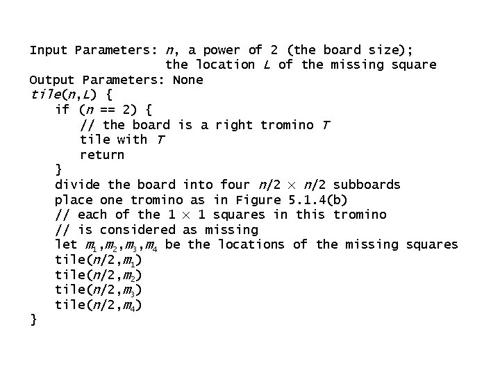
Algorithm 5. 1. 4 Tiling a Deficient Board with Trominoes This algorithm constructs a tiling by trominoes of a deficient n×n board where n is a power of 2.

Input Parameters: n, a power of 2 (the board size); the location L of the missing square Output Parameters: None tile(n, L) { if (n == 2) { // the board is a right tromino T tile with T return } divide the board into four n/2 × n/2 subboards place one tromino as in Figure 5. 1. 4(b) // each of the 1 × 1 squares in this tromino // is considered as missing let m 1, m 2, m 3, m 4 be the locations of the missing squares tile(n/2, m 1) tile(n/2, m 2) tile(n/2, m 3) tile(n/2, m 4) }

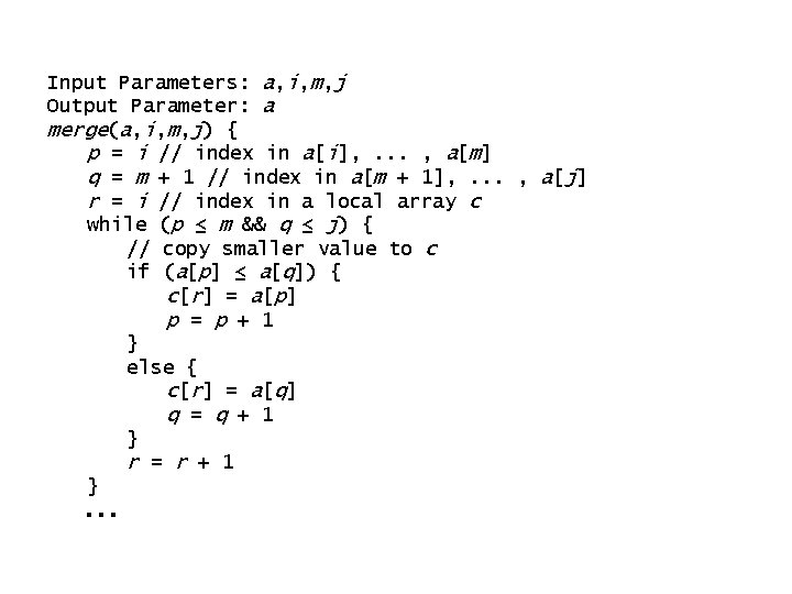
Algorithm 5. 2. 2 Merge This algorithm receives as input indexes i, m, and j, and an array a, where a[i], . . . , a[m] and a[m +1], . . . , a[j] are each sorted in nondecreasing order. These two nondecreasing subarrays are merged into a single nondecreasing array.

Input Parameters: a, i, m, j Output Parameter: a merge(a, i, m, j) { p = i // index in a[i], . . . , a[m] q = m + 1 // index in a[m + 1], . . . , a[j] r = i // index in a local array c while (p ≤ m && q ≤ j) { // copy smaller value to c if (a[p] ≤ a[q]) { c[r] = a[p] p = p + 1 } else { c[r] = a[q] q = q + 1 } r = r + 1 }. . .

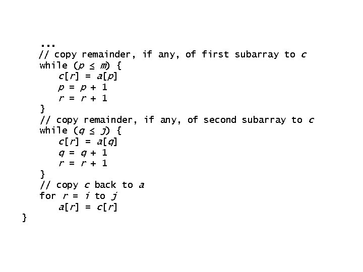
. . . // copy remainder, if any, of first subarray to c while (p ≤ m) { c[r] = a[p] p = p + 1 r = r + 1 } // copy remainder, if any, of second subarray to c while (q ≤ j) { c[r] = a[q] q = q + 1 r = r + 1 } // copy c back to a for r = i to j a[r] = c[r] }

Algorithm 5. 2. 3 Mergesort This algorithm sorts the array a[i], . . . , a[j] in nondecreasing order. It uses the merge algorithm (Algorithm 5. 2. 2). Input Parameters: a, i, j Output Parameter: a mergesort(a, i, j) { // if only one element, just return if (i == j) return // divide a into two nearly equal parts m = (i + j)/2 // sort each half mergesort(a, i, m) mergesort(a, m + 1, j) // merge the two sorted halves merge(a, i, m, j) }

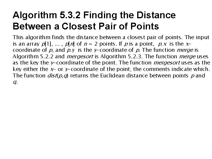
Algorithm 5. 3. 2 Finding the Distance Between a Closest Pair of Points This algorithm finds the distance between a closest pair of points. The input is an array p[1], . . . , p[n] of n = 2 points. If p is a point, p. x is the xcoordinate of p, and p. y is the y-coordinate of p. The function merge is Algorithm 5. 2. 2 and mergesort is Algorithm 5. 2. 3. The function merge uses as the key the y-coordinate of the point. The function mergesort uses as the key either the x- or y-coordinate of the point; the comments indicate which. The function dist(p, q) returns the Euclidean distance between points p and q.

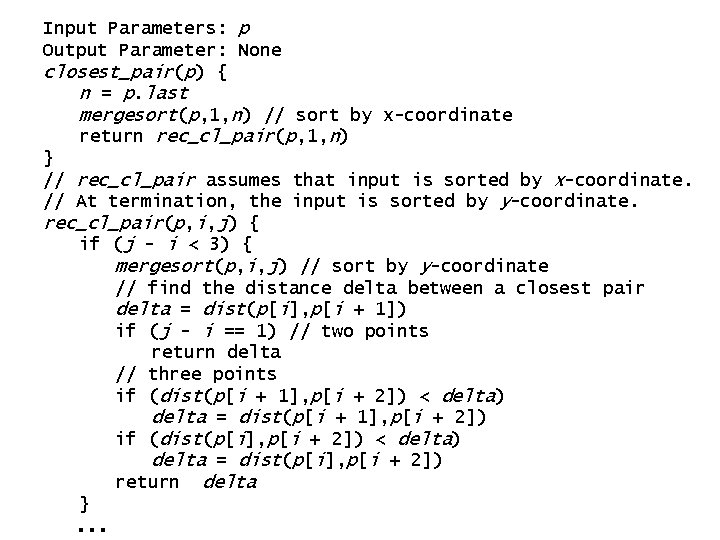
Input Parameters: p Output Parameter: None closest_pair(p) { n = p. last mergesort(p, 1, n) // sort by x-coordinate return rec_cl_pair(p, 1, n) } // rec_cl_pair assumes that input is sorted by x-coordinate. // At termination, the input is sorted by y-coordinate. rec_cl_pair(p, i, j) { if (j - i < 3) { mergesort(p, i, j) // sort by y-coordinate // find the distance delta between a closest pair delta = dist(p[i], p[i + 1]) if (j - i == 1) // two points return delta // three points if (dist(p[i + 1], p[i + 2]) < delta) delta = dist(p[i + 1], p[i + 2]) if (dist(p[i], p[i + 2]) < delta) delta = dist(p[i], p[i + 2]) return delta }. . .

. . . k = (i + j)/ 2 l = p[k]. x delta. L = rec_cl_pair(p, i, k) delta. R = rec_cl_pair(p, k + 1, j) delta = min(delta. L, delta. R) // p[i], . . . , p[k] is now sorted by y-coordinate, and // p[k + 1], . . . , p[j] is now sorted by y-coordinate. merge(p, i, k, j) // p[i], . . . , p[j] is now sorted by y-coordinate. // store points in the vertical strip in v. t = 0 for k = i to j if (p[k]. x > l - delta && p[k]. x < l + delta) { t = t + 1 v[t] = p[k] } // look for closer pairs in the strip by comparing // each point in the strip to the next 7 points. for k = 1 to t - 1 for s = k + 1 to min(t, k + 7) delta = min(delta, dist(v[k], v[s])) return delta }

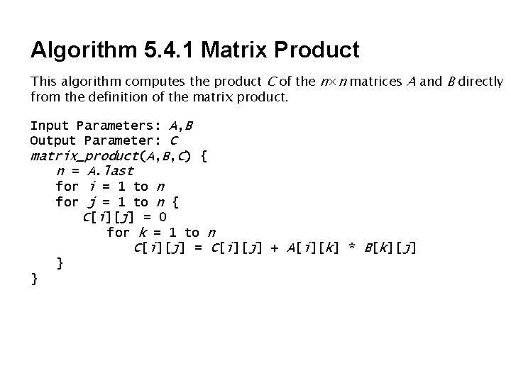
Algorithm 5. 4. 1 Matrix Product This algorithm computes the product C of the n×n matrices A and B directly from the definition of the matrix product. Input Parameters: A, B Output Parameter: C matrix_product(A, B, C) { n = A. last for i = 1 to n for j = 1 to n { C[i][j] = 0 for k = 1 to n C[i][j] = C[i][j] + A[i][k] * B[k][j] } }