The Network Layer NAT IPv 6 Routing Algorithms

The Network Layer: NAT, IPv 6, Routing Algorithms CS 352, Lecture 15, Spring 2020 http: //www. cs. rutgers. edu/~sn 624/352 Srinivas Narayana 1

Course announcements • Take-home mid-term this weekend • Practice problems and review mid-term released soon • Open-book and open-notes, but not open-Internet • Not permitted to search the Internet for answers • No collaboration permitted; all answers and work must be your own • Calculators are allowed • This class will follow absolute grading with generous thresholds • i. e. , no curve, you’re only competing with yourself • We trust you to do the right thing

Review of concepts • Internet Protocol: • Headers: src/dst, upper layer, fragmentation, time to live • Dynamic host configuration protocol (DHCP): • How does an endpoint get its IP address? • Broadcast-based: endpoint asks entire network for answers • DHCP server returns IP address, subnet mask, local DNS server address, gateway router address • Internet Control Message Protocol (ICMP): • Network troubleshooting protocol • Ping: reachability using ICMP echo request and reply • Traceroute: router-level path using ICMP time-exceeded messages and incrementing TTL

Network Address Translation (NAT) How do you survive in a world where names are scarce?

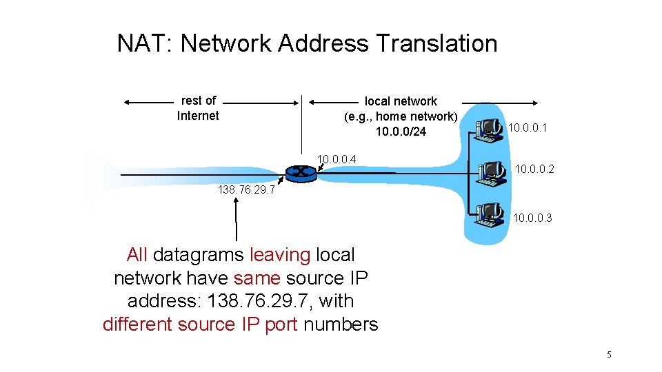
NAT: Network Address Translation rest of Internet local network (e. g. , home network) 10. 0. 0/24 10. 0. 0. 1 10. 0. 0. 2 138. 76. 29. 7 10. 0. 0. 3 All datagrams leaving local network have same source IP address: 138. 76. 29. 7, with different source IP port numbers 5

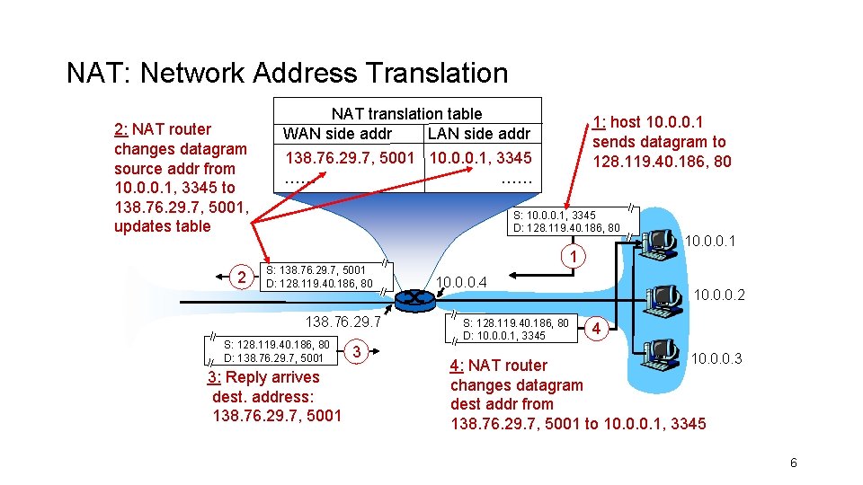
NAT: Network Address Translation 2: NAT router changes datagram source addr from 10. 0. 0. 1, 3345 to 138. 76. 29. 7, 5001, updates table 2 NAT translation table WAN side addr LAN side addr 1: host 10. 0. 0. 1 sends datagram to 128. 119. 40. 186, 80 138. 76. 29. 7, 5001 10. 0. 0. 1, 3345 …… …… S: 10. 0. 0. 1, 3345 D: 128. 119. 40. 186, 80 S: 138. 76. 29. 7, 5001 D: 128. 119. 40. 186, 80 138. 76. 29. 7 S: 128. 119. 40. 186, 80 D: 138. 76. 29. 7, 5001 3: Reply arrives dest. address: 138. 76. 29. 7, 5001 3 1 10. 0. 0. 4 S: 128. 119. 40. 186, 80 D: 10. 0. 0. 1, 3345 10. 0. 0. 1 10. 0. 0. 2 4 10. 0. 0. 3 4: NAT router changes datagram dest addr from 138. 76. 29. 7, 5001 to 10. 0. 0. 1, 3345 6

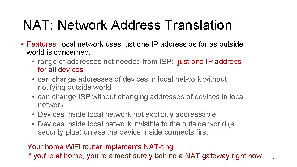
NAT: Network Address Translation • Features: local network uses just one IP address as far as outside world is concerned: • range of addresses not needed from ISP: just one IP address for all devices • can change addresses of devices in local network without notifying outside world • can change ISP without changing addresses of devices in local network • Devices inside local network not explicitly addressable • Devices inside local network invisible to the outside world (a security plus) unless the device inside connects first. Your home Wi. Fi router implements NAT-ting. If you’re at home, you’re almost surely behind a NAT gateway right now. 7

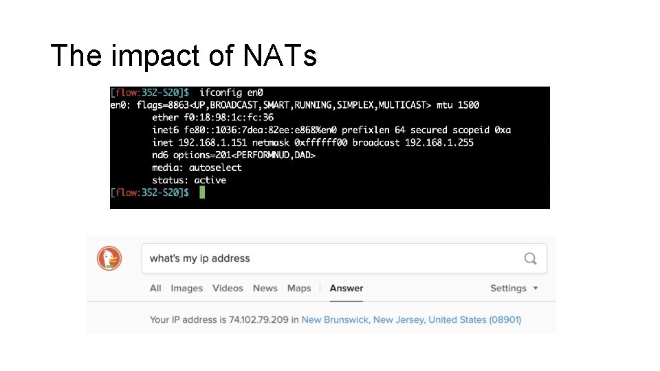
The impact of NATs

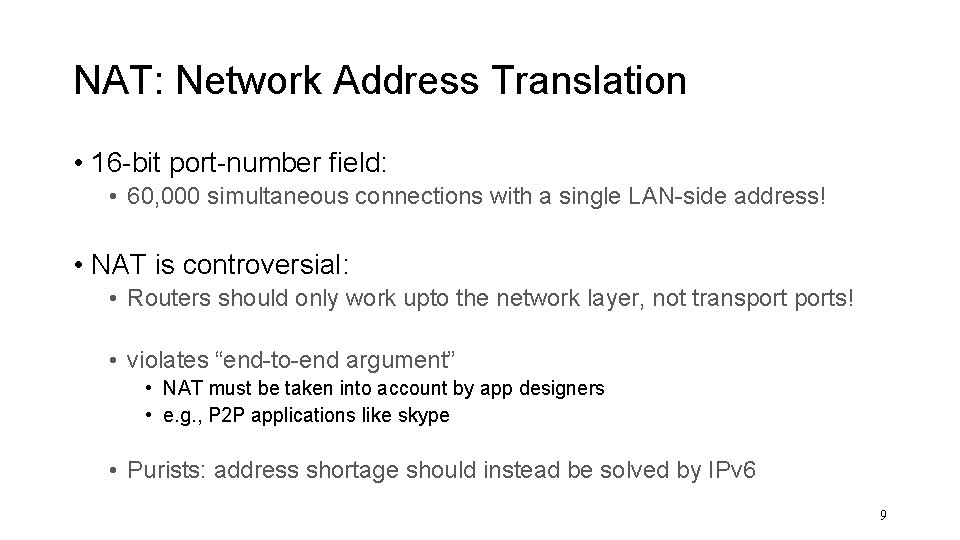
NAT: Network Address Translation • 16 -bit port-number field: • 60, 000 simultaneous connections with a single LAN-side address! • NAT is controversial: • Routers should only work upto the network layer, not transports! • violates “end-to-end argument” • NAT must be taken into account by app designers • e. g. , P 2 P applications like skype • Purists: address shortage should instead be solved by IPv 6 9

Think about… • How do the hosts inside the home network get their IP addresses? • How does your home router get its externally visible IP address?

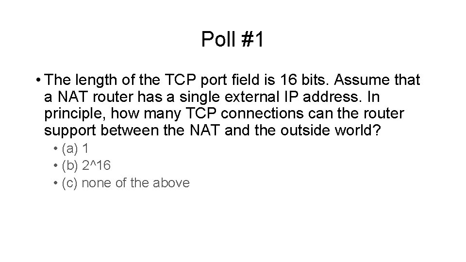
Poll #1 • The length of the TCP port field is 16 bits. Assume that a NAT router has a single external IP address. In principle, how many TCP connections can the router support between the NAT and the outside world? • (a) 1 • (b) 2^16 • (c) none of the above

Internet Protocol v 6 (IPv 6)

Recent Developments: IPv 6 • IPv 4 has limited address space (32 bits) and is running out of addresses. 32 bits are not enough! • More devices: phones, watches, your refrigerator(!), … • Real-time traffic and mobile users are also becoming more common IP version 6 13

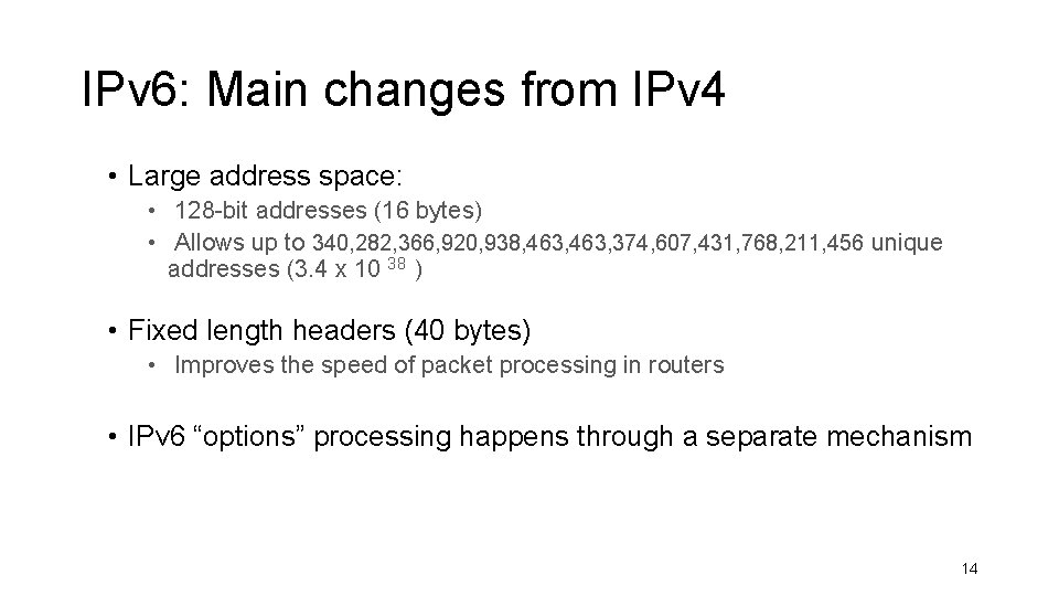
IPv 6: Main changes from IPv 4 • Large address space: • 128 -bit addresses (16 bytes) • Allows up to 340, 282, 366, 920, 938, 463, 374, 607, 431, 768, 211, 456 unique addresses (3. 4 x 10 38 ) • Fixed length headers (40 bytes) • Improves the speed of packet processing in routers • IPv 6 “options” processing happens through a separate mechanism 14

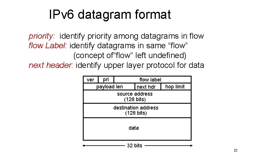
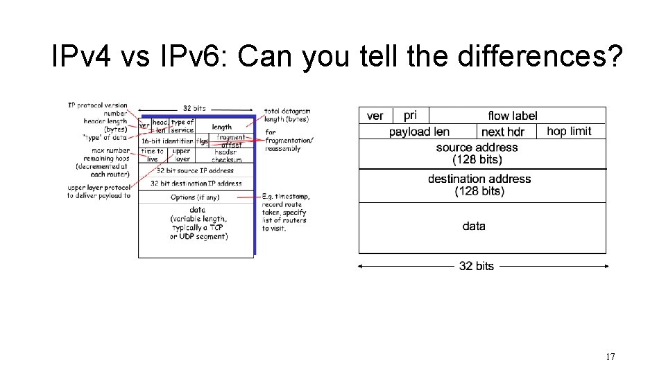
IPv 6 datagram format priority: identify priority among datagrams in flow Label: identify datagrams in same “flow” (concept of“flow” left undefined) next header: identify upper layer protocol for data ver pri flow label hop limit payload len next hdr source address (128 bits) destination address (128 bits) data 32 bits 15

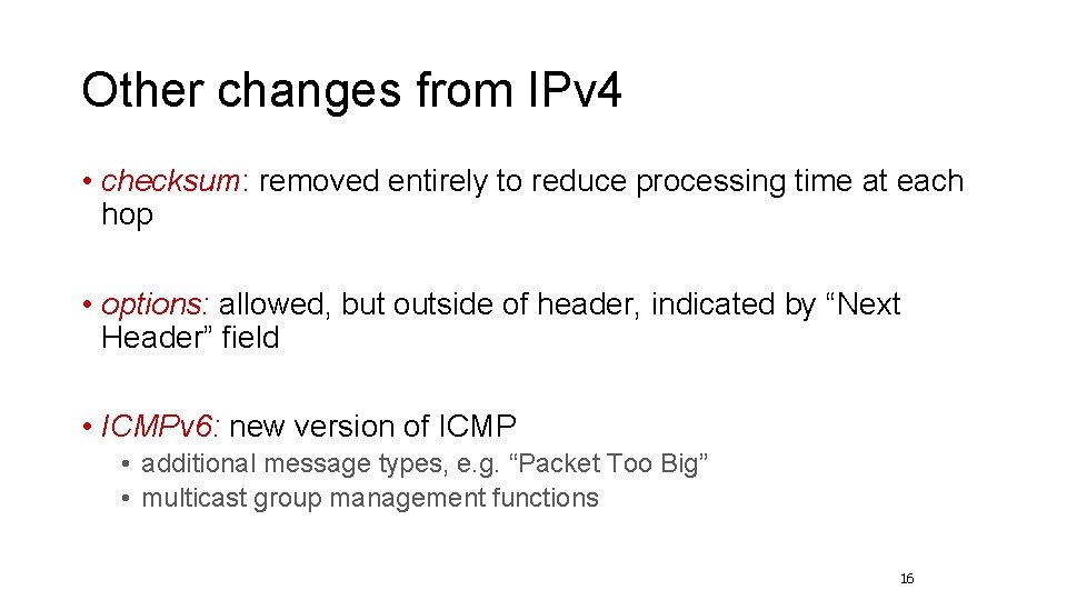
Other changes from IPv 4 • checksum: removed entirely to reduce processing time at each hop • options: allowed, but outside of header, indicated by “Next Header” field • ICMPv 6: new version of ICMP • additional message types, e. g. “Packet Too Big” • multicast group management functions 16

IPv 4 vs IPv 6: Can you tell the differences? 17

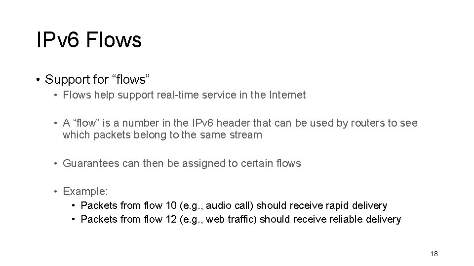
IPv 6 Flows • Support for “flows” • Flows help support real-time service in the Internet • A “flow” is a number in the IPv 6 header that can be used by routers to see which packets belong to the same stream • Guarantees can then be assigned to certain flows • Example: • Packets from flow 10 (e. g. , audio call) should receive rapid delivery • Packets from flow 12 (e. g. , web traffic) should receive reliable delivery 18

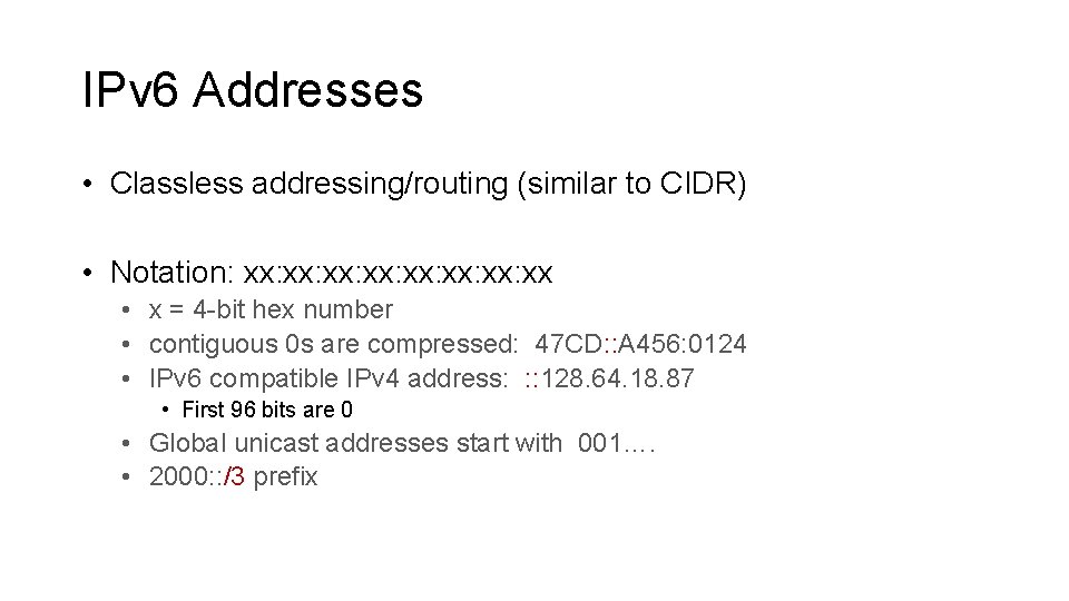
IPv 6 Addresses • Classless addressing/routing (similar to CIDR) • Notation: xx: xx: xx: xx • x = 4 -bit hex number • contiguous 0 s are compressed: 47 CD: : A 456: 0124 • IPv 6 compatible IPv 4 address: : : 128. 64. 18. 87 • First 96 bits are 0 • Global unicast addresses start with 001…. • 2000: : /3 prefix

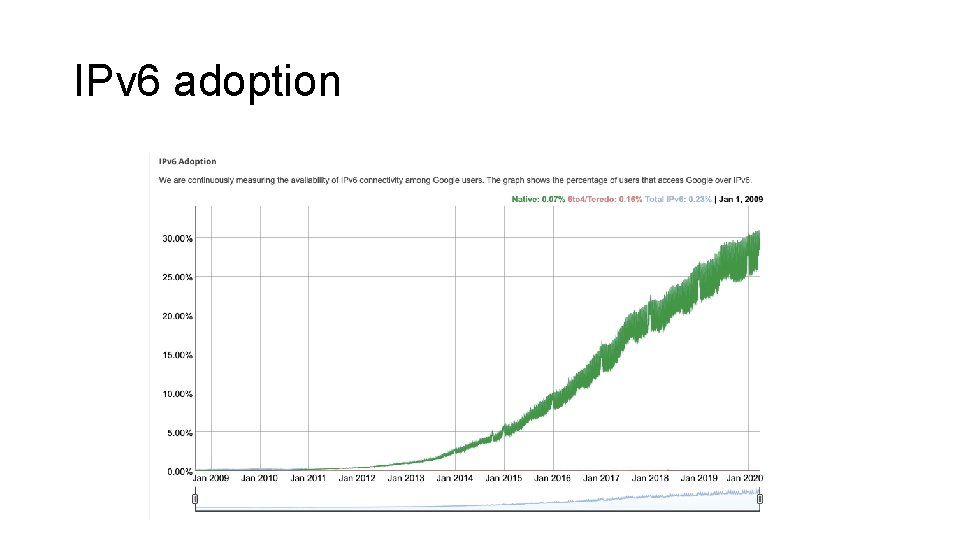
IPv 6 adoption

IPv 6: Adoption • Google: ~1/3 of clients access services via IPv 6 (Apr 2020) • Long (long!) time for deployment, use • 20 years and counting! • Think of application-level changes in last 20 years: WWW, Facebook, Skype, video streaming, AR, telesurgery, … • Why? 21

Poll #2 • What’s the primary difference between IPv 4 and IPv 6? • (a) Larger address space • (b) Fixed-length, fewer headers by default • (c) No fragmentation • (d) All of the above

Routing Protocols How do we design a “Google Maps” navigator for the Internet?

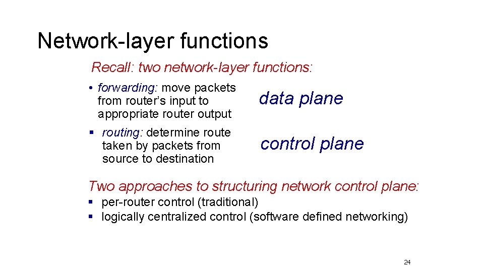
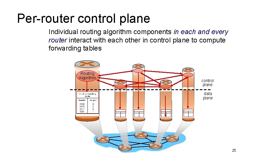
Network-layer functions Recall: two network-layer functions: • forwarding: move packets from router’s input to appropriate router output data plane § routing: determine route taken by packets from source to destination control plane Two approaches to structuring network control plane: § per-router control (traditional) § logically centralized control (software defined networking) 24

Per-router control plane Individual routing algorithm components in each and every router interact with each other in control plane to compute forwarding tables Routing Algorithm control plane data plane 25

Routing protocols Routing protocol goal: determine “good” paths (equivalently, routes), from sending hosts to receiving host, through network of routers • path: sequence of routers packets will traverse in going from given initial source host to given final destination host • “good”: least “cost”, “fastest”, “least congested” • routing: a “top-10” networking challenge! 26

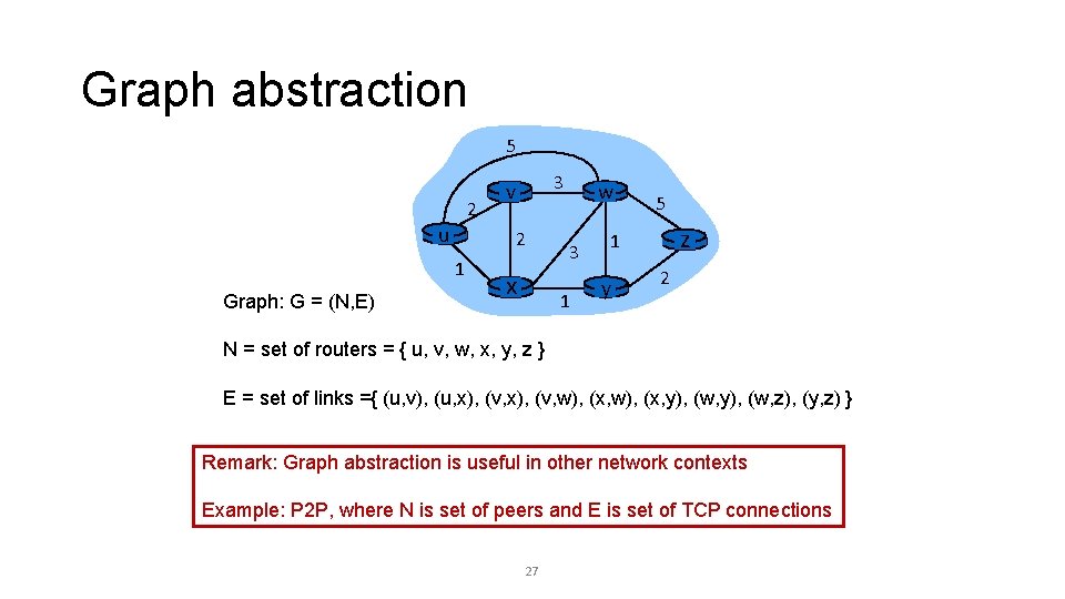
Graph abstraction 5 2 u 2 1 Graph: G = (N, E) 3 v w 3 x 1 5 z 1 y 2 N = set of routers = { u, v, w, x, y, z } E = set of links ={ (u, v), (u, x), (v, w), (x, y), (w, z), (y, z) } Remark: Graph abstraction is useful in other network contexts Example: P 2 P, where N is set of peers and E is set of TCP connections 27

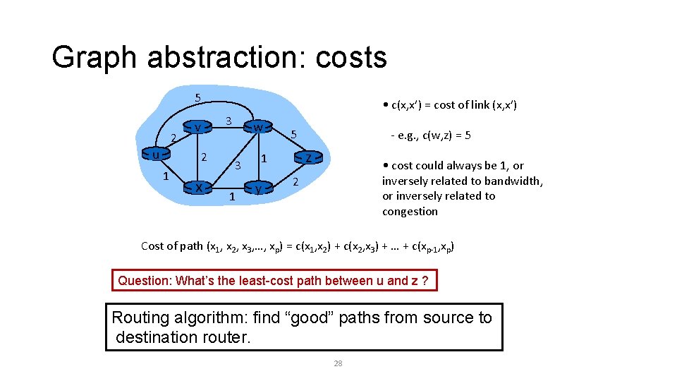
Graph abstraction: costs 5 2 u v 2 1 x • c(x, x’) = cost of link (x, x’) 3 w 3 1 5 z 1 y - e. g. , c(w, z) = 5 • cost could always be 1, or inversely related to bandwidth, or inversely related to congestion 2 Cost of path (x 1, x 2, x 3, …, xp) = c(x 1, x 2) + c(x 2, x 3) + … + c(xp-1, xp) Question: What’s the least-cost path between u and z ? Routing algorithm: find “good” paths from source to destination router. 28

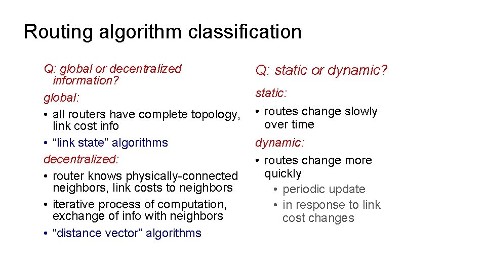
Routing algorithm classification Q: global or decentralized information? global: • all routers have complete topology, link cost info • “link state” algorithms decentralized: • router knows physically-connected neighbors, link costs to neighbors • iterative process of computation, exchange of info with neighbors • “distance vector” algorithms Q: static or dynamic? static: • routes change slowly over time dynamic: • routes change more quickly • periodic update • in response to link cost changes

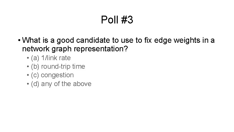
Poll #3 • What is a good candidate to use to fix edge weights in a network graph representation? • (a) 1/link rate • (b) round-trip time • (c) congestion • (d) any of the above

Link State Algorithms

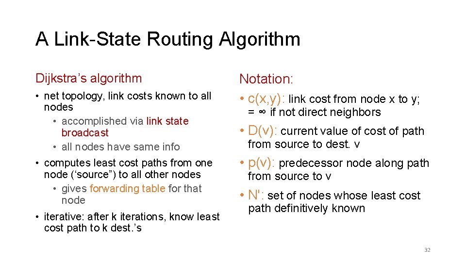
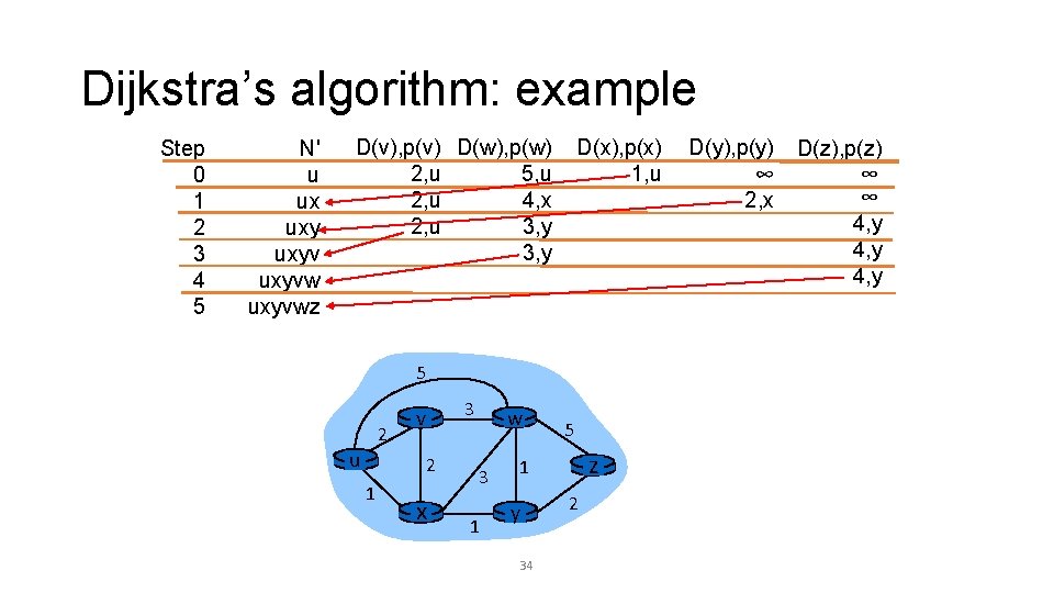
A Link-State Routing Algorithm Dijkstra’s algorithm • net topology, link costs known to all nodes • accomplished via link state broadcast • all nodes have same info • computes least cost paths from one node (‘source”) to all other nodes • gives forwarding table for that node • iterative: after k iterations, know least cost path to k dest. ’s Notation: • c(x, y): link cost from node x to y; = ∞ if not direct neighbors • D(v): current value of cost of path from source to dest. v • p(v): predecessor node along path from source to v • N': set of nodes whose least cost path definitively known 32

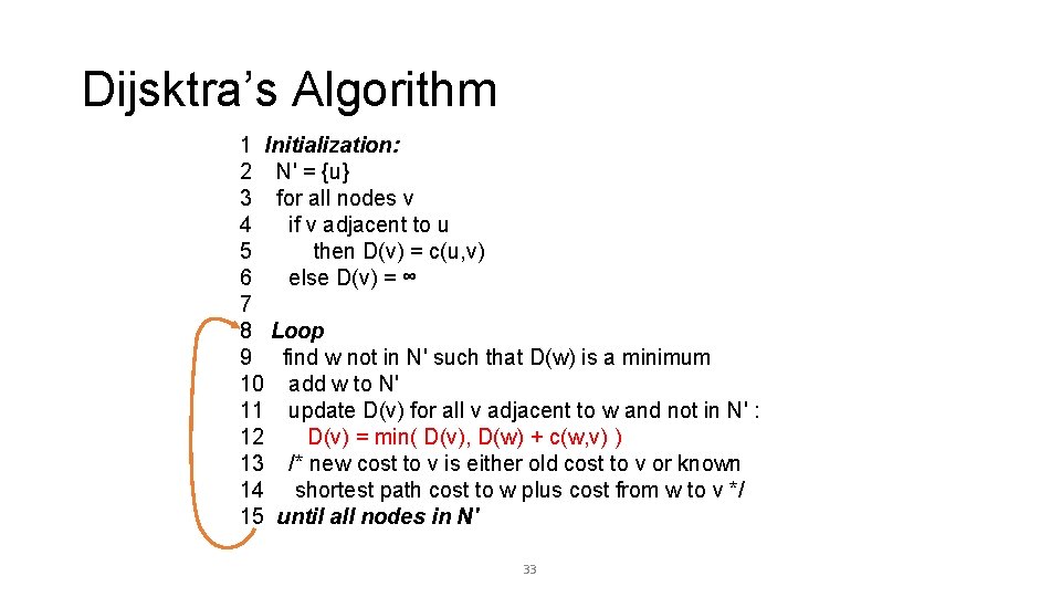
Dijsktra’s Algorithm 1 Initialization: 2 N' = {u} 3 for all nodes v 4 if v adjacent to u 5 then D(v) = c(u, v) 6 else D(v) = ∞ 7 8 Loop 9 find w not in N' such that D(w) is a minimum 10 add w to N' 11 update D(v) for all v adjacent to w and not in N' : 12 D(v) = min( D(v), D(w) + c(w, v) ) 13 /* new cost to v is either old cost to v or known 14 shortest path cost to w plus cost from w to v */ 15 until all nodes in N' 33

Dijkstra’s algorithm: example Step 0 1 2 3 4 5 N' u ux uxyvwz D(v), p(v) D(w), p(w) 2, u 5, u 2, u 4, x 2, u 3, y D(x), p(x) 1, u 5 2 u v 2 1 x 3 w 3 1 5 z 1 y 34 2 D(y), p(y) ∞ 2, x D(z), p(z) ∞ ∞ 4, y

Poll #4 • Link-state information of a router is sent to all routers before computing shortest paths in a link-state protocol. • (a) true • (b) false

Poll #5 • Link-state protocols don’t compute shortest paths when there are cycles in the network topology. • (a) true • (b) false

Distance Vector Algorithms

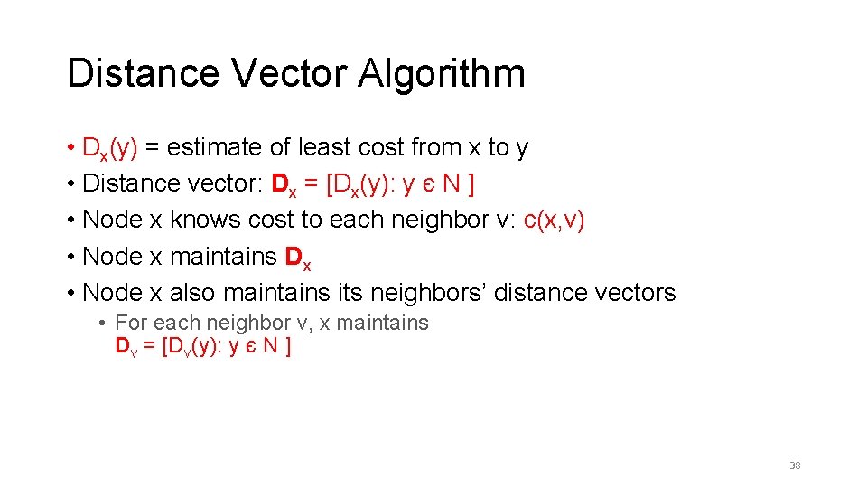
Distance Vector Algorithm • Dx(y) = estimate of least cost from x to y • Distance vector: Dx = [Dx(y): y є N ] • Node x knows cost to each neighbor v: c(x, v) • Node x maintains Dx • Node x also maintains its neighbors’ distance vectors • For each neighbor v, x maintains Dv = [Dv(y): y є N ] 38

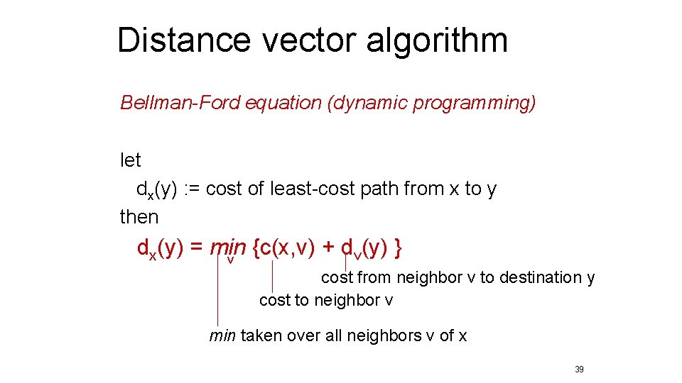
Distance vector algorithm Bellman-Ford equation (dynamic programming) let dx(y) : = cost of least-cost path from x to y then dx(y) = min {c(x, v) + d (y) } v v cost from neighbor v to destination y cost to neighbor v min taken over all neighbors v of x 39

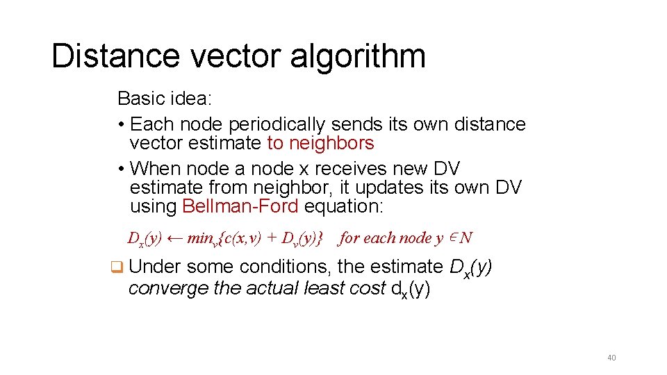
Distance vector algorithm Basic idea: • Each node periodically sends its own distance vector estimate to neighbors • When node a node x receives new DV estimate from neighbor, it updates its own DV using Bellman-Ford equation: Dx(y) ← minv{c(x, v) + Dv(y)} for each node y ∊ N q Under some conditions, the estimate Dx(y) converge the actual least cost dx(y) 40

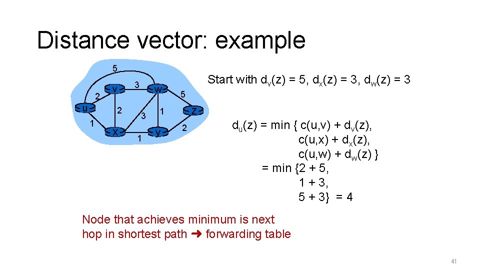
Distance vector: example 5 2 u v 2 1 x 3 w 3 1 Start with dv(z) = 5, dx(z) = 3, dw(z) = 3 5 z 1 y 2 du(z) = min { c(u, v) + dv(z), c(u, x) + dx(z), c(u, w) + dw(z) } = min {2 + 5, 1 + 3, 5 + 3} = 4 Node that achieves minimum is next hop in shortest path ➜ forwarding table 41

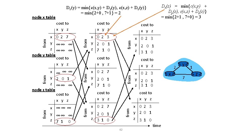
from x ∞∞ ∞ y ∞∞ ∞ z 7 1 0 cost to x y z x 0 2 3 y 2 0 1 z 7 1 0 x 0 2 3 y 2 0 1 z 3 1 0 from cost to x y z x 0 2 7 y 2 0 1 z 7 1 0 x 0 2 3 y 2 0 1 z 3 1 0 from x ∞ ∞ ∞ y 2 0 1 z ∞∞ ∞ node z table cost to x y z from x 0 2 7 y ∞∞ ∞ z ∞∞ ∞ node y table cost to x y z from cost to x y z x 0 2 7 y 2 0 1 z 3 1 0 x 0 2 3 y 2 0 1 z 3 1 0 from node x table Dx(z) = min{c(x, y) + Dy(z), c(x, z) + Dz(z)} = min{2+1 , 7+0} = 3 Dx(y) = min{c(x, y) + Dy(y), c(x, z) + Dz(y)} = min{2+0 , 7+1} = 2 42 time 2 x y 7 1 z

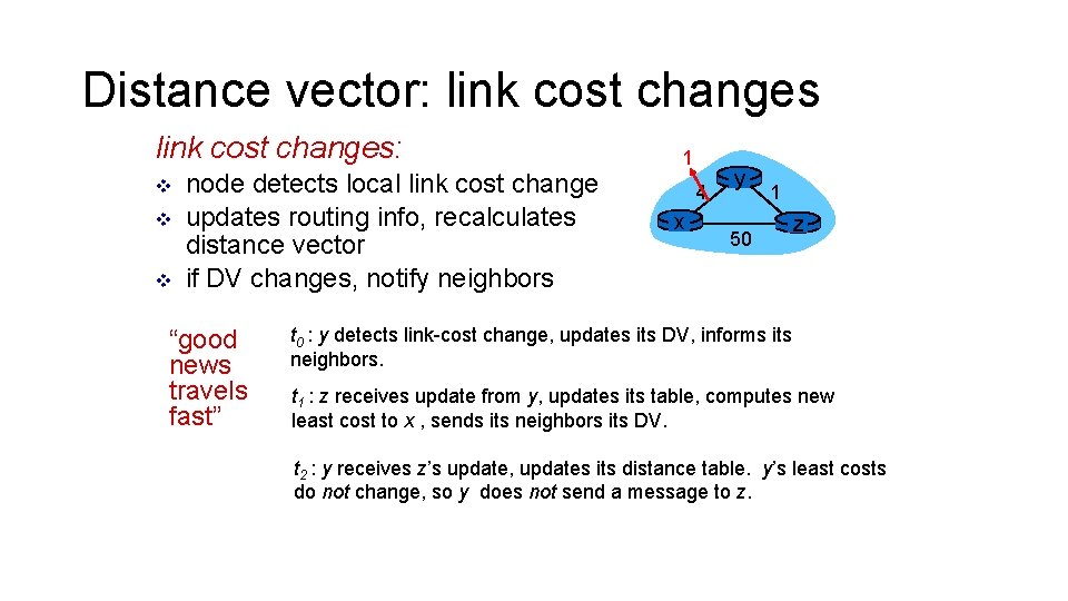
Distance vector: link cost changes: v v v node detects local link cost change updates routing info, recalculates distance vector if DV changes, notify neighbors “good news travels fast” 1 4 x y 1 50 z t 0 : y detects link-cost change, updates its DV, informs its neighbors. t 1 : z receives update from y, updates its table, computes new least cost to x , sends its neighbors its DV. t 2 : y receives z’s update, updates its distance table. y’s least costs do not change, so y does not send a message to z.

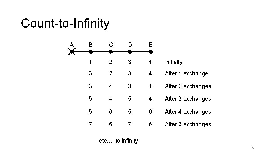
Problem: Count-to-Infinity • With distance vector routing, good news travels fast, but bad news travels slowly • When a router goes down, it takes can take a really long time before all the other routers become aware of it 44

Count-to-Infinity A B C D E 1 2 3 4 Initially 3 2 3 4 After 1 exchange 3 4 After 2 exchanges 5 4 After 3 exchanges 5 6 After 4 exchanges 7 6 After 5 exchanges etc… to infinity 45

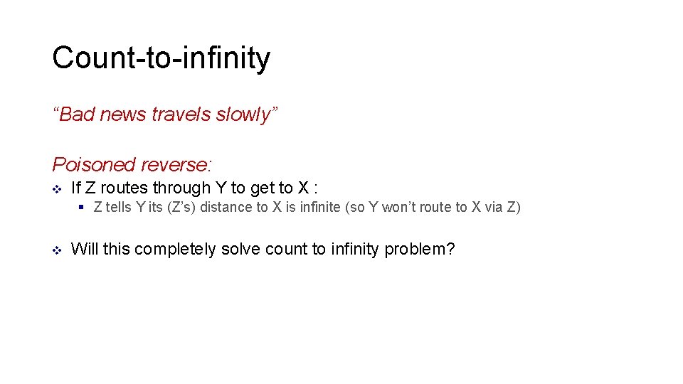
Count-to-infinity “Bad news travels slowly” Poisoned reverse: v If Z routes through Y to get to X : § Z tells Y its (Z’s) distance to X is infinite (so Y won’t route to X via Z) v Will this completely solve count to infinity problem?

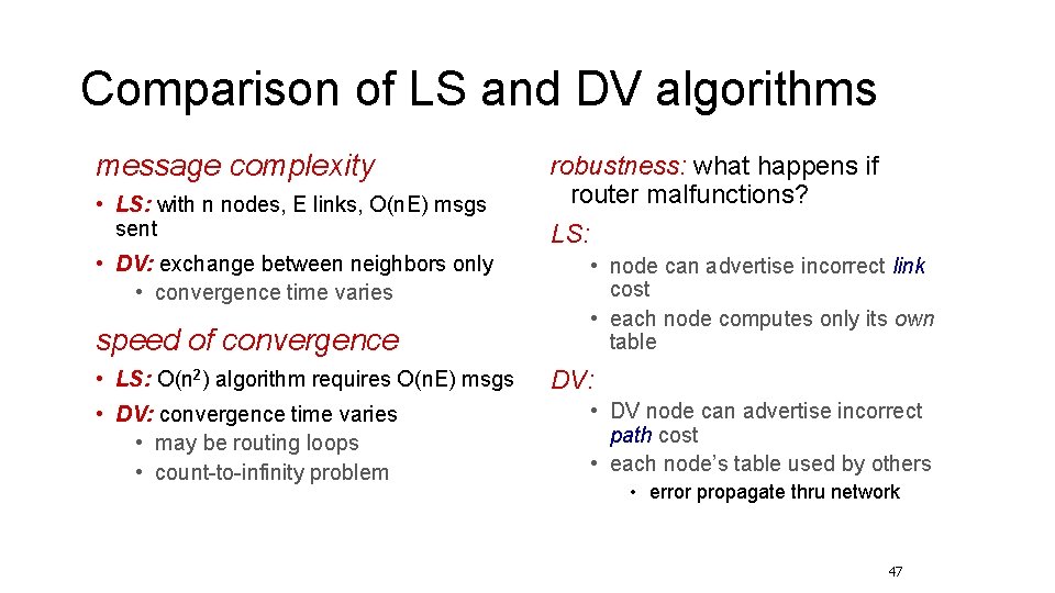
Comparison of LS and DV algorithms message complexity • LS: with n nodes, E links, O(n. E) msgs sent • DV: exchange between neighbors only • convergence time varies speed of convergence • LS: O(n 2) algorithm requires O(n. E) msgs • DV: convergence time varies • may be routing loops • count-to-infinity problem robustness: what happens if router malfunctions? LS: • node can advertise incorrect link cost • each node computes only its own table DV: • DV node can advertise incorrect path cost • each node’s table used by others • error propagate thru network 47

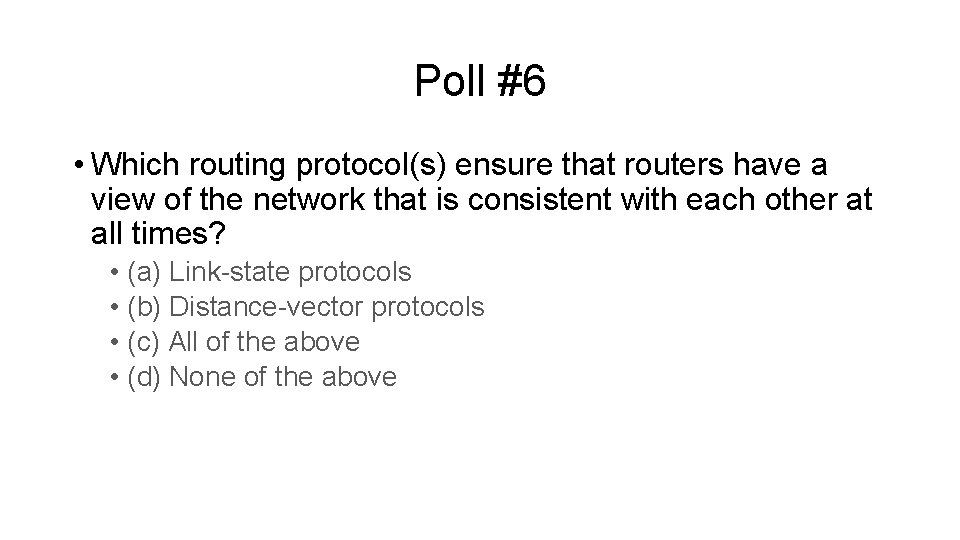
Poll #6 • Which routing protocol(s) ensure that routers have a view of the network that is consistent with each other at all times? • (a) Link-state protocols • (b) Distance-vector protocols • (c) All of the above • (d) None of the above

Routing protocols are widely deployed • OSPF: a link-state protocol • “Open Shortest Path First” • IS-IS, nearly identical to OSPF • RIP: a distance-vector protocol • LS and DV deployed inside an autonomous system • Additional tricks to scale the protocols with network size: • Areas; Hierarchy • “Border routers” that summarize each area • Next lecture: Routing across autonomous systems