Divide and Conquer 1 2 3 4 5

Divide and Conquer 1. 2. 3. 4. 5. Merge sort and quick sort Binary search Multiplication of large integers Strassen’s Matrix Multiplication Closest pair problem

Expected Outcomes Students should be able to § Explain the idea and steps of divide and conquer § Explain the ideas of mergesort and quicksort § Analyze the time complexity of mergesort and quicksort algorithms in the best, worst and average cases

Divide and Conquer A successful military strategy long before it became an algorithm design strategy § Coalition uses divide-conquer plan in Fallujah, Iraq. – By Rowan Scarborough and Bill Gertz, THE WASHINGTON TIMES Example: Your instructor give you a 500 -question assignment today and ask you to turn it in the tomorrow. What should you do?

Three Steps of The Divide and Conquer Approach The most well known algorithm design strategy Divide the problem into two or more smaller subproblems. Conquer the subproblems by solving them recursively. Combine the solutions to the subproblems into the solutions to the original problem.

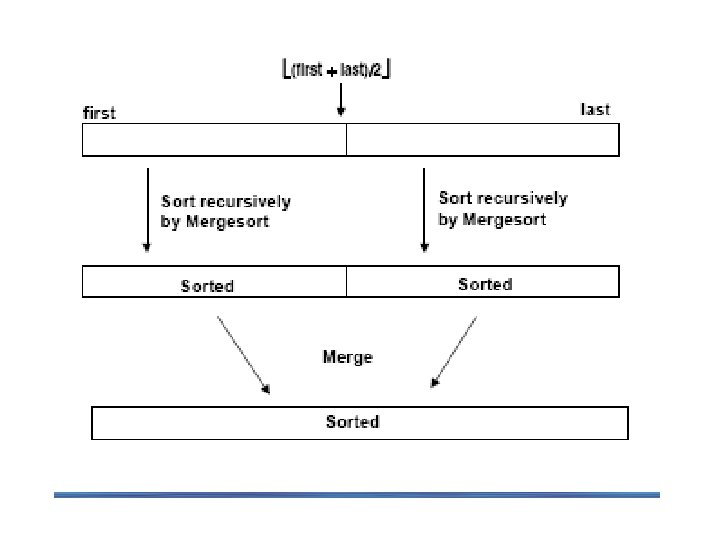
A typical case of divide and conquer technique

An Example: Calculating a 0 + a 1 + … + an-1 Let us consider the problem of computing the sum of n numbers a 0 + a 1 + … + an-1. If n>1, we can divide the problem into two instances of the same problem: to compute the sum of first n/2 numbers and to compute sum of the remaining n/2 numbers. We can add these two values to get the sum in question: a 0 + … + an-1 = (a 0 + … + an/2 – 1 ) + (an/2 + … + an-1 ) it is worth keeping in mind that divide-conquer technique is ideally suited for parallel computations, in which each sub-problem can be solved simultaneously by its own processor.

An Example: Calculating a 0 + a 1 + … + an-1 More generally, an instance of size n can be divided into several instances of size n/b, with a of them needing to be solved. Here a and b are constants (a>=1 and b>1). Assuming that size n is power of b, to simplify our analysis we get the following recurrence for the running time T(n): T(n) = a. T(n/b) + f(n), This equation is called the general divide-and-conquer recurrence. Where f(n) is function that accounts for the time spent on dividing the problem into smaller ones and on combining their solutions. The efficiency analysis of many divide-and-conquer algorithms is greatly simplified by the following theorem.

Master Theorem The same results hold with O and Ω notations, too. For example, the recurrence equation for the number of additions A(n) made by the divide-and-conquer summation algorithm on inputs of size n = 2 k is, A(n) = 2 A(n/2) + 1. Thus, for this example, a=2, b=2, and d=0; hence, since a > bd, A(n) Θ(nlogba) = Θ(nlog 22) = Θ(n).

Idea of Mergesort is a perfect example of a successful application of the divide-and-conquer technique. n Divide: divide array A[0. . n-1] in two about equal halves and make copies of each half in arrays B and C n Conquer: l If number of elements in B and C is 1, directly solve it l Sort arrays B and C recursively n Combine: Merge sorted arrays B and C into array A l Repeat the following until no elements remain in one of the arrays: - l compare the first elements in the remaining unprocessed portions of the arrays B and C copy the smaller of the two into A, while incrementing the index indicating the unprocessed portion of that array Once all elements in one of the arrays are processed, copy the remaining unprocessed elements from the other array into A.

The Mergesort Algorithm

The Merge Algorithm

Mergesort Examples The operation of the algorithm on the list is illustrated in figure below: 83297154 § Try to answer the following questions? – – How many key comparisons needed? How much extra memory needed? Is the algorithm an in-place algorithm? Is the algorithm stable?

Analysis of Mergesort Assuming for simplicity that n is a power of 2, the recurrence relation for the number of basic operations (key comparisons): § T(n) = 2 T(n/2) + (n) Worst case and best case § T(n) = 2 T(n/2) + n-1 § T(n) = 2 T(n/2) + n/2 All cases: Θ(n log n) Space complexity: (n), not in-place Stable

The Divide, Conquer and Combine Steps in Quicksort is another important sorting algorithm that is based on the divide-andconquer approach. Unlike mergesort, which divides its input’s elements according to their position in the array, quicksort divides them according to their value. Divide: Partition array A[l. . r] into 2 subarrays, A[l. . s-1] and A[s+1. . r] such that each element of the first array is ≤A[s] and each element of the second array is ≥ A[s]. (computing the index of s is part of partition. ) § Implication: A[s] will be in its final position in the sorted array. Conquer: Sort the two subarrays A[l. . s-1] and A[s+1. . r] by recursive calls to quicksort Combine: No work is needed, because A[s] is already in its correct place after the partition is done, and the two subarrays have been sorted.

Quicksort Select a pivot w. r. t. whose value we are going to divide the list. (typically, p = A[l]) Rearrange the list so that all the elements in the first s positions are smaller than or equal to the pivot and all the elements in the remaining n-s positions are larger than or equal to the pivot p A[i] p Exchange the pivot with the last element in the first sublist(i. e. , ≤ sublist) – the pivot is now in its final position Sort the two sublists recursively using quicksort.

The Quicksort Algorithm ALGORITHM Quicksort(A[l. . r]) //Sorts a subarray by quicksort //Input: A subarray A[l. . r] of A[0. . n-1], defined by its left and right indices l and r //Output: The subarray A[l. . r] sorted in nondecreasing order if l < r s Partition (A[l. . r]) // s is a split position Quicksort(A[l. . s-1]) Quicksort(A[s+1. . r]

Partitioning Algorithm Can ‘=’ be removed from ‘ ’ and ‘ ’? Number of comparisons: n or n + 1

Quicksort Example 15 22 13 27 22 10 20 25 • Try to answer the following questions? How much extra memory needed? Is the algorithm an in-place algorithm? Is the algorithm stable? How many key comparisons needed? Should introduce an extra element with enough value for A[0, n-1], that is, A[n] = . Consider why?

Another Partitioning Algorithm Partition(A[l, r]) p = A[l ] Pivot. Loc = l for i = l+1 to r do if A[ i ] < p then Pivot. Loc = Pivot. Loc+ 1 if Pivot. Loc <> i then Swap( A[ Pivot. Loc ], A[ i ] ) end if end for Swap(A[ Pivot. Loc ], A[ l ] ) // move pivotinto correct place return Pivot. Loc Number of comparisons: n-1 for all

Efficiency of Quicksort Based on whether the partitioning is balanced. Best case: split in the middle — Θ( n log n) § C(n) = 2 C(n/2) + Θ(n) //2 subproblems of size n/2 each Worst case: sorted array! — Θ( n 2) § C(n) = C(n-1) + Θ(n) //2 subproblems of size 0 and n-1 respectively § Is there any other possible array with worst case comparisons? Average case: random arrays — Θ( n log n) By the second partition algorithm

Improvements: § better pivot selection: median-of-three partitioning § switch to insertion sort on small subfiles § elimination of recursion These combine to 20 -25% improvement

Binary Search an Iterative Algorithm Very efficient algorithm for searching in sorted array: K vs A[0]. . . A[m]. . . A[n-1] If K = A[m], stop (successful search); otherwise, continue searching by the same method in A[0. . m-1] if K < A[m] and in A[m+1. . n-1] if K > A[m] Binary search is clearly based on recursive idea, it can be easily implemented as a nonrecursive algorithm, too. Here is pesudocode for this nonrecursive version: ALGORITHM Binary. Search(A[0. . n-1], K) l 0; r n-1 while l r do // l and r crosses over can’t find K m (l+r)/2 if K = A[m] return m //the key is found else if K < A[m] r m-1 //the key is on the left half of the array else l m+1 // the key is on the right half of the array return -1

Binary Search – a Recursive Algorithm ALGORITHM Binary. Search. Recur(A[0. . n-1], l, r, K) if l > r return – 1 else m (l + r) / 2 if K = A[m] return m else if K < A[m] return Binary. Search. Recur(A[0. . n-1], l, m-1, K) else return Binary. Search. Recur(A[0. . n-1], m+1, r, K)

Analysis of Binary Search Let us find the number of key comparisons in the Worst-Case (successful /fail) Cw (n). The worst case inputs include all arrays that do not contain a given search key. Since after one comparison the algorithm faces the same situation but for an array half the size, we get the following recurrence relation: Cw (n) = Cw( n/2 ) + 1 for n>1, Cw (1) = 1 ----- (4. 2) For simplicity n = 2 k so, Cw(2 k) = k + 1 = log 2 n +1 ---------(4. 3) Equation (4. 3) for n = 2 k can be tweaked to get a solution valid for an positive integer n: Cw(n) = log 2 n +1 = log 2(n+1) ---------(4. 4)

This is VERY fast: e. g. , Cw(106) = 20 by applying equation 4. 4 Best-case: successful Cb (n) = 1, fail Cb (n) = log 2 n +1 Average-case: The average number of key comparisons made by binary search is only smaller than that in the worst case: Cavg (n) ≈ log 2 n More accurate, average comparison in a successful and unsuccessful search are Cavg (n) ≈ log 2 n – 1 and Cavg (n) ≈ log 2 (n+1)

Remarks on Binary Search Optimal for searching in a sorted array Limitations: must be a sorted array (not linked list) Bad (degenerate) example of divide-and-conquer Has a continuous counterpart called bisection method for solving equations in one unknown f(x) = 0 (see Sec. 12. 4)

Binary Tree Traversals Definitions § A binary tree T is defined as a finite set of nodes that is either empty or consists of a root and two disjoint binary trees TL and TR called, respectively, the left and right subtree of the root. § The height of a tree is defined as the length of the longest path from the root to a leaf. Problem: find the height of a binary tree.

Find the Height of a Binary Tree ALGORITHM Height(T) //Computes recursively the height of a binary tree //Input: A binary tree T //Output: The height of T if T = return – 1 else return max{Height(TL), Height(TR)} + 1 Analysis: Number of comparisons of a tree T with : 2 n + 1 Number of comparisons of height is the same as number of additions: A(n(T)) = A(n(TL)) + A(n(TR)) +1 for n>0, A(0) = 0 The solution is A(n) = n

Binary Tree Traversals– preorder, inorder, and postorder traversal Binary tee traversal: visit all nodes of a binary tree recursively. Write a recursive preorder binary tree traversal algorithm. Algorithm Preorder(T) //Implement the preorder traversal of a binary tree //Input: Binary tree T (with labeled vertices) //Output: Node labels listed in preorder if T ‡ write label of T’s root Preorder(TL) Preorder(TR)

Closest-Pair by Divide-and-Conquer Step 1 Divide the points given into two subsets S 1 and S 2 by a vertical line x = c so that half the points lie to the left or on the line and half the points lie to the right or on the line.

Closest Pair by Divide-and-Conquer Step 2 Find recursively the closest pairs for the left and right subsets. Step 3 Set d = min{d 1, d 2} We can limit our attention to the points in the symmetric vertical strip of width 2 d as possible closest pair. Let C 1 and C 2 be the subsets of points in the left subset S 1 and of the right subset S 2, respectively, that lie in this vertical strip. The points in C 1 and C 2 are stored in increasing order of their y coordinates, which is maintained by merging during the execution of the next step. Step 4 For every point P(x, y) in C 1, we inspect points in C 2 that may be closer to P than d. There can be no more than 6 such points (because d ≤ d 2)!

Closest Pair by Divide-and-Conquer: Worst Case The worst case scenario is depicted below:

Efficiency of the Closest-Pair Algorithm Running time of the algorithm is described by T(n) = 2 T(n/2) + M(n), where M(n) O(n) By the Master Theorem (with a = 2, b = 2, d = 1) T(n) O(n log n) The most efficient algorithm!