ALGORITHM TYPES Greedy Divide and Conquer Dynamic Programming

ALGORITHM TYPES • Greedy, Divide and Conquer, Dynamic Programming, Random Algorithms, and Backtracking. • Note the general strategy from the examples. • The classification is neither exhaustive (there may be more) nor mutually exclusive (one may combine). • We are now emphasizing design of algorithms, not data structures.

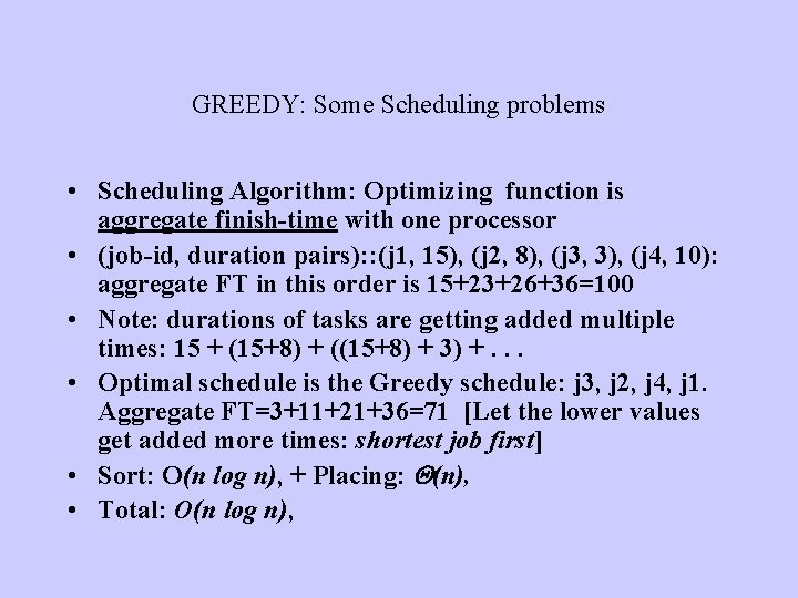
GREEDY: Some Scheduling problems • Scheduling Algorithm: Optimizing function is aggregate finish-time with one processor • (job-id, duration pairs): : (j 1, 15), (j 2, 8), (j 3, 3), (j 4, 10): aggregate FT in this order is 15+23+26+36=100 • Note: durations of tasks are getting added multiple times: 15 + (15+8) + ((15+8) + 3) +. . . • Optimal schedule is the Greedy schedule: j 3, j 2, j 4, j 1. Aggregate FT=3+11+21+36=71 [Let the lower values get added more times: shortest job first] • Sort: O(n log n), + Placing: (n), • Total: O(n log n),

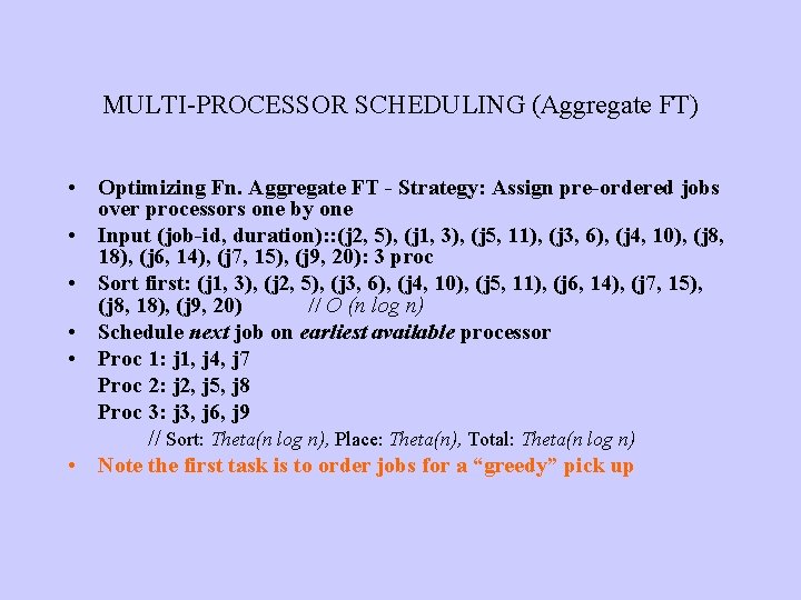
MULTI-PROCESSOR SCHEDULING (Aggregate FT) • Optimizing Fn. Aggregate FT - Strategy: Assign pre-ordered jobs over processors one by one • Input (job-id, duration): : (j 2, 5), (j 1, 3), (j 5, 11), (j 3, 6), (j 4, 10), (j 8, 18), (j 6, 14), (j 7, 15), (j 9, 20): 3 proc • Sort first: (j 1, 3), (j 2, 5), (j 3, 6), (j 4, 10), (j 5, 11), (j 6, 14), (j 7, 15), (j 8, 18), (j 9, 20) // O (n log n) • Schedule next job on earliest available processor • Proc 1: j 1, j 4, j 7 Proc 2: j 2, j 5, j 8 Proc 3: j 3, j 6, j 9 // Sort: Theta(n log n), Place: Theta(n), Total: Theta(n log n) • Note the first task is to order jobs for a “greedy” pick up

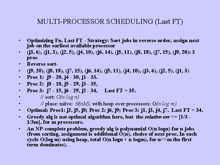
MULTI-PROCESSOR SCHEDULING (Last FT) • • • Optimizing Fn. Last FT - Strategy: Sort jobs in reverse order, assign next job on the earliest available processor (j 3, 6), (j 1, 3), (j 2, 5), (j 4, 10), (j 6, 14), (j 5, 11), (j 8, 18), (j 7, 15), (j 9, 20): 3 proc Reverse sort(j 9, 20), (j 8, 18), (j 7, 15), (j 6, 14), (j 5, 11), (j 4, 10), (j 3, 6), (j 2, 5), (j 1, 3) Proc 1: j 9 - 20, j 4 - 30, j 1 - 33. Proc 2: j 8 - 18, j 5 - 29, j 3 - 35, Proc 3: j 7 - 15, j 6 - 29, j 2 - 34, Last FT = 35. // sort: O(n log n) // place: naïve: (n. M), with heap over processors: O(n log m) Optimal: Proc 1: j 2, j 5, j 8; Proc 2: j 6, j 9; Proc 3: j 1, j 3, j 4, j 7. Last FT = 34. Greedy alg is not optimal algorithm here, but the relative err <= [1/3 1/3 m], for m processors. An NP-complete problem, greedy alg is polynomial O(n logn) for n jobs (from sorting, assignment is additional O(n), choice of next proc. In each cycle O(log m) using heap, total O(n logn + n logm), for n>>m the first term dominates).

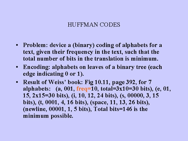
HUFFMAN CODES • Problem: device a (binary) coding of alphabets for a text, given their frequency in the text, such that the total number of bits in the translation is minimum. • Encoding: alphabets on leaves of a binary tree (each edge indicating 0 or 1). • Result of Weiss’ book: Fig 10. 11, page 392, for 7 alphabets: (a, 001, freq=10, total=3 x 10=30 bits), (e, 01, 15, 2 x 15=30 bits), (i, 10, 12, 24 bits), (s, 00000, 3, 15 bits), (t, 0001, 4, 16 bits), (space, 11, 13, 26 bits), (newline, 00001, 1, 5 bits), Total bits=146 is the minimum possible.

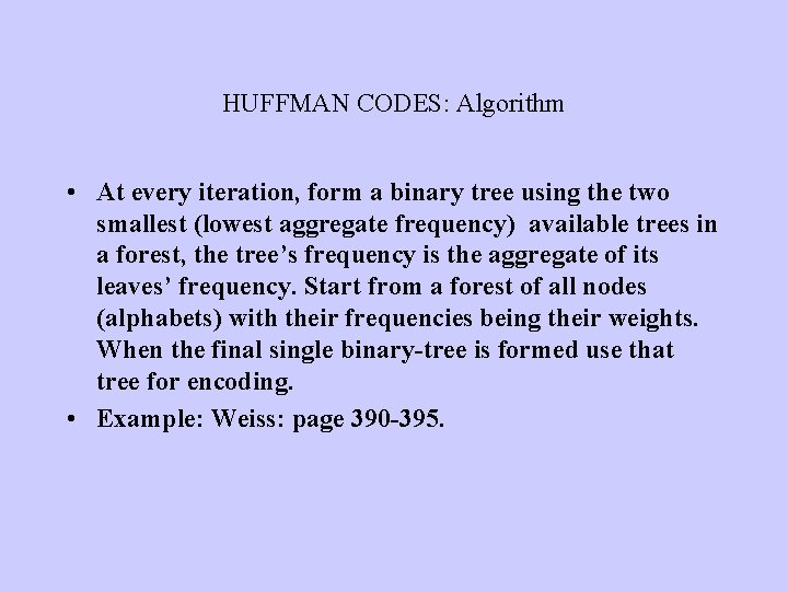
HUFFMAN CODES: Algorithm • At every iteration, form a binary tree using the two smallest (lowest aggregate frequency) available trees in a forest, the tree’s frequency is the aggregate of its leaves’ frequency. Start from a forest of all nodes (alphabets) with their frequencies being their weights. When the final single binary-tree is formed use that tree for encoding. • Example: Weiss: page 390 -395.

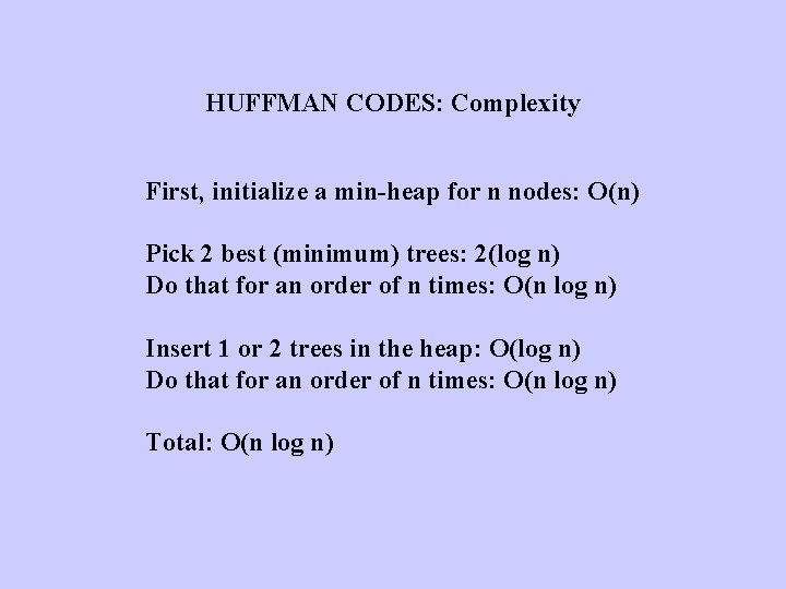
HUFFMAN CODES: Complexity First, initialize a min-heap for n nodes: O(n) Pick 2 best (minimum) trees: 2(log n) Do that for an order of n times: O(n log n) Insert 1 or 2 trees in the heap: O(log n) Do that for an order of n times: O(n log n) Total: O(n log n)

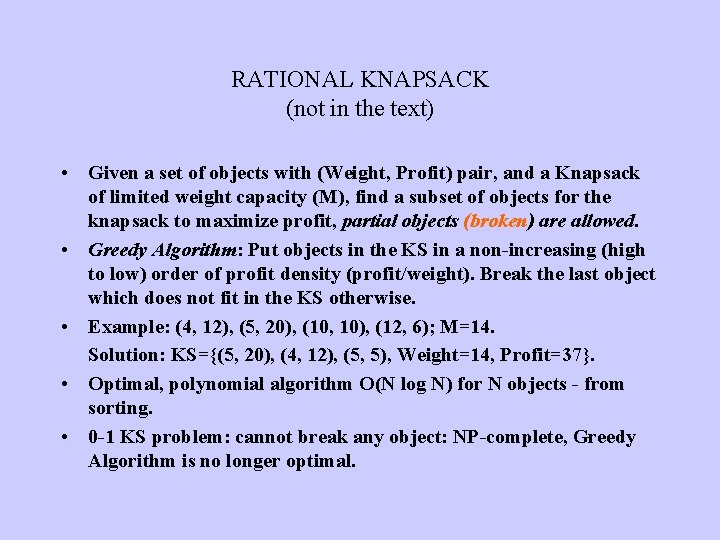
RATIONAL KNAPSACK (not in the text) • Given a set of objects with (Weight, Profit) pair, and a Knapsack of limited weight capacity (M), find a subset of objects for the knapsack to maximize profit, partial objects (broken) are allowed. • Greedy Algorithm: Put objects in the KS in a non-increasing (high to low) order of profit density (profit/weight). Break the last object which does not fit in the KS otherwise. • Example: (4, 12), (5, 20), (10, 10), (12, 6); M=14. Solution: KS={(5, 20), (4, 12), (5, 5), Weight=14, Profit=37}. • Optimal, polynomial algorithm O(N log N) for N objects - from sorting. • 0 -1 KS problem: cannot break any object: NP-complete, Greedy Algorithm is no longer optimal.

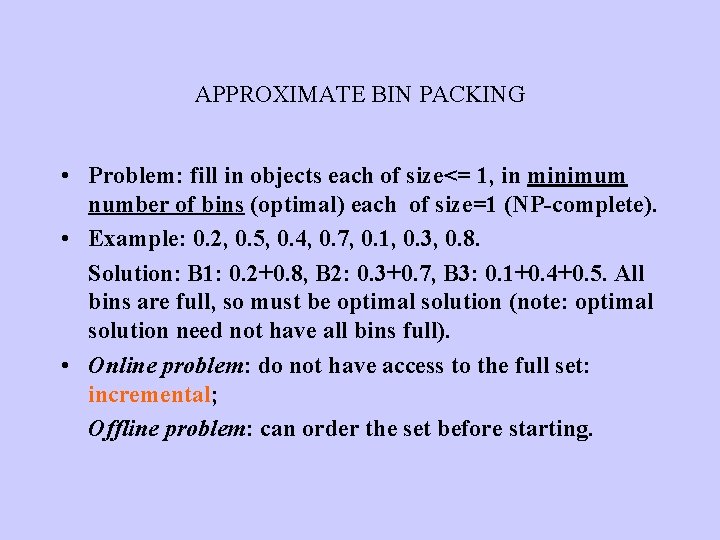
APPROXIMATE BIN PACKING • Problem: fill in objects each of size<= 1, in minimum number of bins (optimal) each of size=1 (NP-complete). • Example: 0. 2, 0. 5, 0. 4, 0. 7, 0. 1, 0. 3, 0. 8. Solution: B 1: 0. 2+0. 8, B 2: 0. 3+0. 7, B 3: 0. 1+0. 4+0. 5. All bins are full, so must be optimal solution (note: optimal solution need not have all bins full). • Online problem: do not have access to the full set: incremental; Offline problem: can order the set before starting.

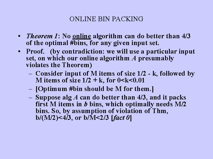
ONLINE BIN PACKING • Theorem 1: No online algorithm can do better than 4/3 of the optimal #bins, for any given input set. • Proof. (by contradiction: we will use a particular input set, on which our online algorithm A presumably violates the Theorem) – Consider input of M items of size 1/2 - k, followed by M items of size 1/2 + k, for 0<k<0. 01 – [Optimum #bin should be M for them. ] – Suppose alg A can do better than 4/3, and it packs first M items in b bins, which optimally needs M/2 bins. So, by assumption of violation of Thm, b/(M/2)<4/3, or b/M<2/3 [fact 0]

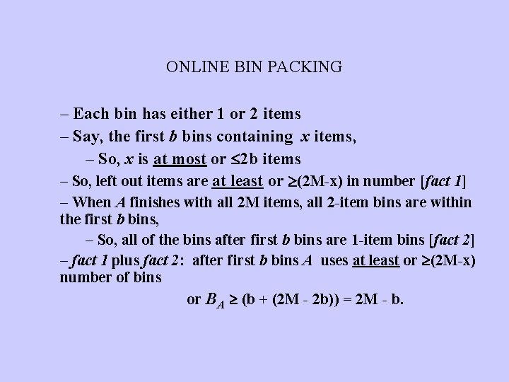
ONLINE BIN PACKING – Each bin has either 1 or 2 items – Say, the first b bins containing x items, – So, x is at most or 2 b items – So, left out items are at least or (2 M-x) in number [fact 1] – When A finishes with all 2 M items, all 2 -item bins are within the first b bins, – So, all of the bins after first b bins are 1 -item bins [fact 2] – fact 1 plus fact 2: after first b bins A uses at least or (2 M-x) number of bins or BA (b + (2 M - 2 b)) = 2 M - b.

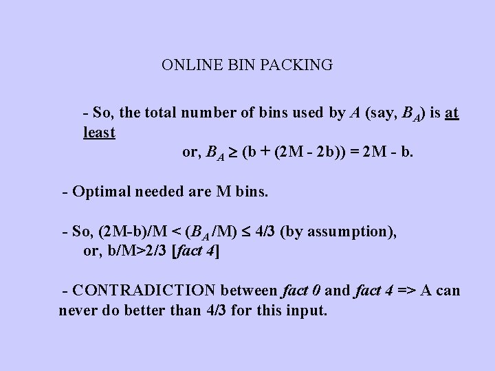
ONLINE BIN PACKING - So, the total number of bins used by A (say, BA) is at least or, BA (b + (2 M - 2 b)) = 2 M - b. - Optimal needed are M bins. - So, (2 M-b)/M < (BA /M) 4/3 (by assumption), or, b/M>2/3 [fact 4] - CONTRADICTION between fact 0 and fact 4 => A can never do better than 4/3 for this input.

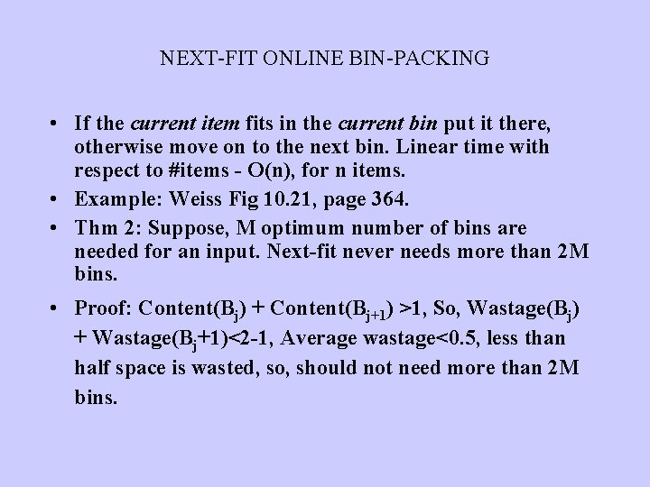
NEXT-FIT ONLINE BIN-PACKING • If the current item fits in the current bin put it there, otherwise move on to the next bin. Linear time with respect to #items - O(n), for n items. • Example: Weiss Fig 10. 21, page 364. • Thm 2: Suppose, M optimum number of bins are needed for an input. Next-fit never needs more than 2 M bins. • Proof: Content(Bj) + Content(Bj+1) >1, So, Wastage(Bj) + Wastage(Bj+1)<2 -1, Average wastage<0. 5, less than half space is wasted, so, should not need more than 2 M bins.

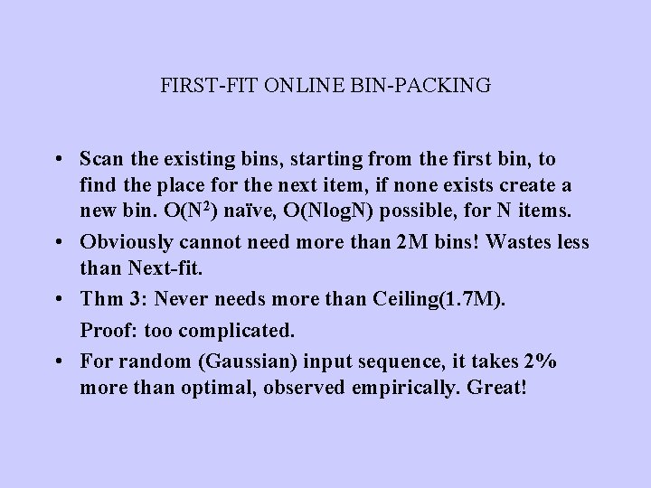
FIRST-FIT ONLINE BIN-PACKING • Scan the existing bins, starting from the first bin, to find the place for the next item, if none exists create a new bin. O(N 2) naïve, O(Nlog. N) possible, for N items. • Obviously cannot need more than 2 M bins! Wastes less than Next-fit. • Thm 3: Never needs more than Ceiling(1. 7 M). Proof: too complicated. • For random (Gaussian) input sequence, it takes 2% more than optimal, observed empirically. Great!

BEST-FIT ONLINE BIN-PACKING • Scan to find the tightest spot for each item (reduce wastage even further than the previous algorithms), if none exists create a new bin. • Does not improve over First-Fit in worst case in optimality, but does not take more worst-case time either! Easy to code.

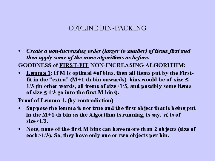
OFFLINE BIN-PACKING • Create a non-increasing order (larger to smaller) of items first and then apply some of the same algorithms as before. GOODNESS of FIRST-FIT NON-INCREASING ALGORITHM: • Lemma 1: If M is optimal #of bins, then all items put by the Firstfit in the “extra” (M+1 -th bin onwards) bins would be of size 1/3 (in other words, all items of size>1/3, and possibly some items of size 1/3 go into the first M bins). Proof of Lemma 1. (by contradiction) • Suppose the lemma is not true and the first object that is being put in the M+1 -th bin as the Algorithm is running, is say, si, is of size>1/3. • Note, none of the first M bins can have more than 2 objects (size of each>1/3). So, they have only one or two objects per bin.

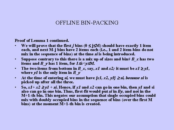
OFFLINE BIN-PACKING Proof of Lemma 1 continued. • We will prove that the first j bins (0 j M) should have exactly 1 item each, and next M-j bins have 2 items each (i. e. , 1 and 2 item-bins do not mix in the sequence of bins) at the time si is being introduced. • Suppose contrary to this there is a mix up of sizes and bin# B_x has two items and B_y has 1 item, for 1 x<y M. • The two items from bottom in B_x, say, x 1 and x 2; it must be x 1 y 1, where y 1 is the only item in B_y • At the time of entering si, we must have {x 1, x 2, y 1} si, because si is picked up after all the three. • So, x 1+ x 2 y 1 + si. Hence, if x 1 and x 2 can go in one bin, then y 1 and si also can go in one bin. Thus, first-fit would put si in By, and not in the M+1 -th bin. This negates our assumption that single occupied bins could mix with doubly occupied bins in the sequence of bins (over the first M bins) at the moment M+1 -th bin is created.

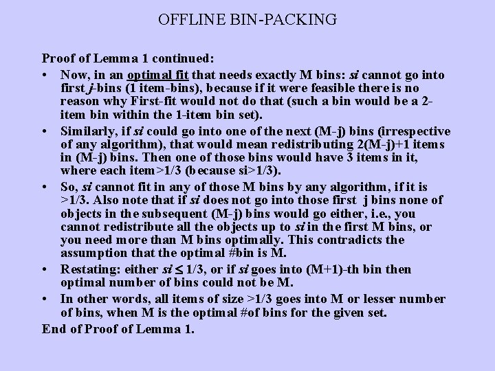
OFFLINE BIN-PACKING Proof of Lemma 1 continued: • Now, in an optimal fit that needs exactly M bins: si cannot go into first j-bins (1 item-bins), because if it were feasible there is no reason why First-fit would not do that (such a bin would be a 2 item bin within the 1 -item bin set). • Similarly, if si could go into one of the next (M-j) bins (irrespective of any algorithm), that would mean redistributing 2(M-j)+1 items in (M-j) bins. Then one of those bins would have 3 items in it, where each item>1/3 (because si>1/3). • So, si cannot fit in any of those M bins by any algorithm, if it is >1/3. Also note that if si does not go into those first j bins none of objects in the subsequent (M-j) bins would go either, i. e. , you cannot redistribute all the objects up to si in the first M bins, or you need more than M bins optimally. This contradicts the assumption that the optimal #bin is M. • Restating: either si 1/3, or if si goes into (M+1)-th bin then optimal number of bins could not be M. • In other words, all items of size >1/3 goes into M or lesser number of bins, when M is the optimal #of bins for the given set. End of Proof of Lemma 1.

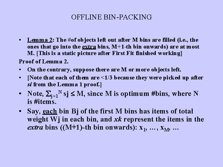
OFFLINE BIN-PACKING • Lemma 2: The #of objects left out after M bins are filled (i. e. , the ones that go into the extra bins, M+1 -th bin onwards) are at most M. [This is a static picture after First Fit finished working] Proof of Lemma 2. • On the contrary, suppose there are M or more objects left. • [Note that each of them are <1/3 because they were picked up after si from the Lemma 1 proof. ] • Note, j=1 N sj M, since M is optimum #bins, where N is #items. • Say, each bin Bj of the first M bins has items of total weight Wj in each bin, and xk represent the items in the extra bins ((M+1)-th bin onwards): x 1, …, x. M, …

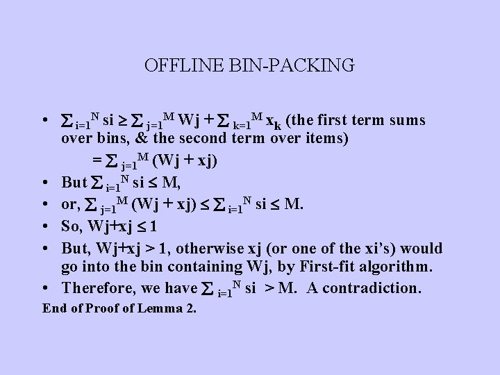
OFFLINE BIN-PACKING • i=1 N si j=1 M Wj + k=1 M xk (the first term sums over bins, & the second term over items) = j=1 M (Wj + xj) • But i=1 N si M, • or, j=1 M (Wj + xj) i=1 N si M. • So, Wj+xj 1 • But, Wj+xj > 1, otherwise xj (or one of the xi’s) would go into the bin containing Wj, by First-fit algorithm. • Therefore, we have i=1 N si > M. A contradiction. End of Proof of Lemma 2.

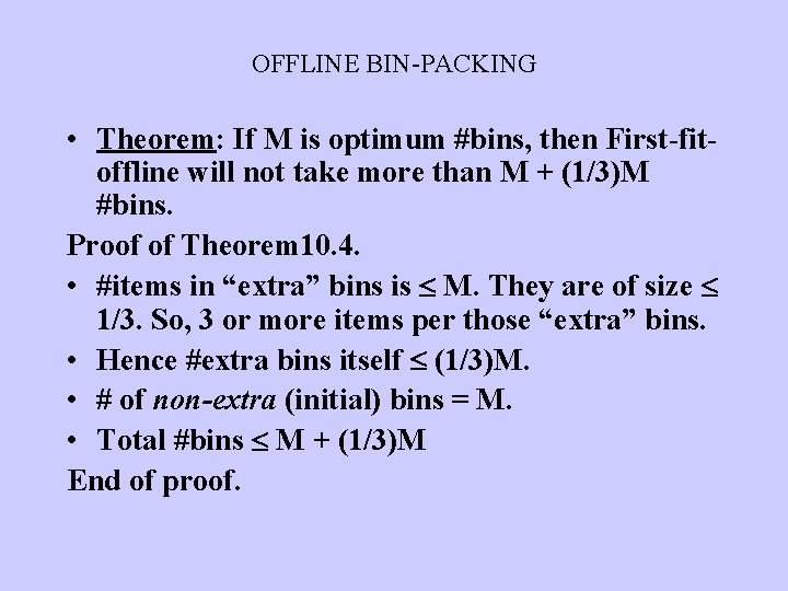
OFFLINE BIN-PACKING • Theorem: If M is optimum #bins, then First-fitoffline will not take more than M + (1/3)M #bins. Proof of Theorem 10. 4. • #items in “extra” bins is M. They are of size 1/3. So, 3 or more items per those “extra” bins. • Hence #extra bins itself (1/3)M. • # of non-extra (initial) bins = M. • Total #bins M + (1/3)M End of proof.

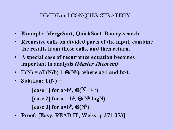
DIVIDE and CONQUER STRATEGY • Example: Merge. Sort, Quick. Sort, Binary-search. • Recursive calls on divided parts of the input, combine the results from those calls, and then return. • A special case of recurrence equation becomes important in analysis (Master Theorem) • T(N) = a. T(N/b) + (Nk), where a 1 and b>1. • Solution: T(N) = [case 1] for a>bk, (N logba) [case 2] for a = bk, (Nk log. N) [case 3] for a<bk, (Nk) • Proof: [Easy, READ IT, Weiss: p 371 -373]

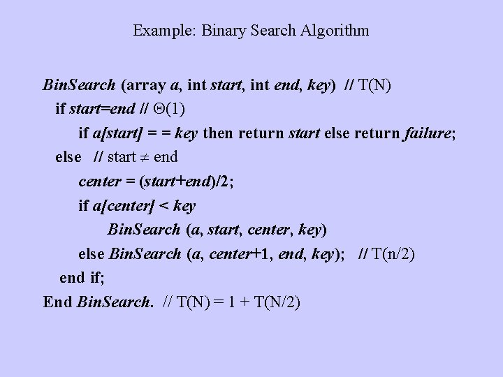
Example: Binary Search Algorithm Bin. Search (array a, int start, int end, key) // T(N) if start=end // (1) if a[start] = = key then return start else return failure; else // start end center = (start+end)/2; if a[center] < key Bin. Search (a, start, center, key) else Bin. Search (a, center+1, end, key); // T(n/2) end if; End Bin. Search. // T(N) = 1 + T(N/2)

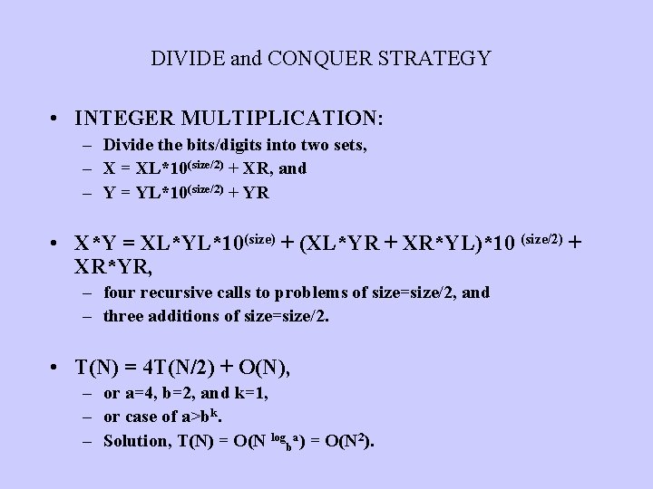
DIVIDE and CONQUER STRATEGY • INTEGER MULTIPLICATION: – Divide the bits/digits into two sets, – X = XL*10(size/2) + XR, and – Y = YL*10(size/2) + YR • X*Y = XL*YL*10(size) + (XL*YR + XR*YL)*10 (size/2) + XR*YR, – four recursive calls to problems of size=size/2, and – three additions of size=size/2. • T(N) = 4 T(N/2) + O(N), – or a=4, b=2, and k=1, – or case of a>bk. – Solution, T(N) = O(N logba) = O(N 2).

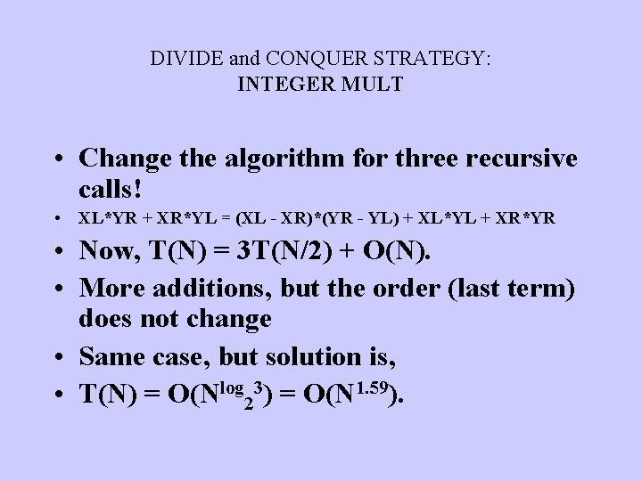
DIVIDE and CONQUER STRATEGY: INTEGER MULT • Change the algorithm for three recursive calls! • XL*YR + XR*YL = (XL - XR)*(YR - YL) + XL*YL + XR*YR • Now, T(N) = 3 T(N/2) + O(N). • More additions, but the order (last term) does not change • Same case, but solution is, • T(N) = O(Nlog 23) = O(N 1. 59).

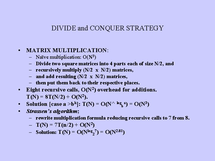
DIVIDE and CONQUER STRATEGY • MATRIX MULTIPLICATION: – – – Naïve multiplication: O(N 3) Divide two square matrices into 4 parts each of size N/2, and recursively multiply (N/2 x N/2) matrices, and add resulting (N/2 x N/2) matrices, then put them back to their respective places. • Eight recursive calls, O(N 2) overhead for additions. T(N) = 8 T(N/2) + O(N 2). • Solution [case a >bk]: T(N) = O(N^ logba) = O(N 3) • Strassen’s algorithm; – rewrite multiplication formula reducing recursive calls to 7 from 8. – T(N) = 7 T(n/2) + O(N 2) – Solution: T(N) = O(Nlog 27) = O(N 2. 81)

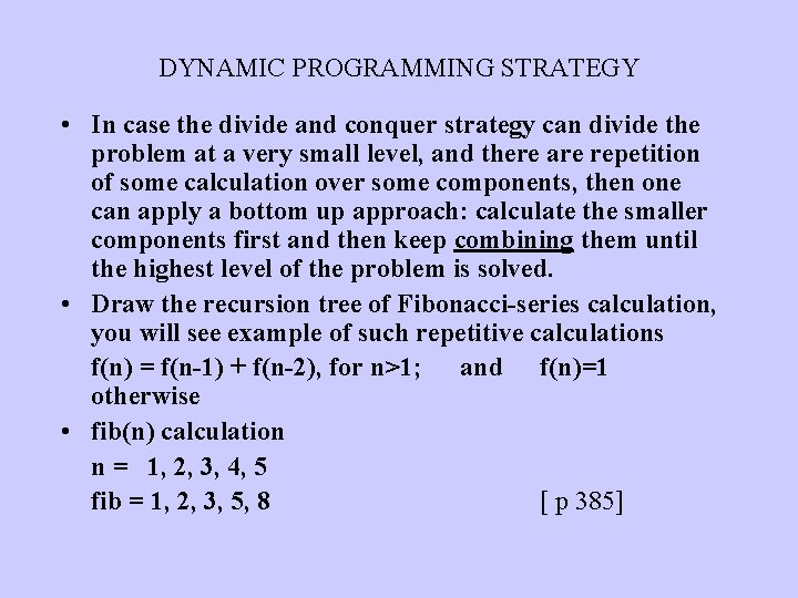
DYNAMIC PROGRAMMING STRATEGY • In case the divide and conquer strategy can divide the problem at a very small level, and there are repetition of some calculation over some components, then one can apply a bottom up approach: calculate the smaller components first and then keep combining them until the highest level of the problem is solved. • Draw the recursion tree of Fibonacci-series calculation, you will see example of such repetitive calculations f(n) = f(n-1) + f(n-2), for n>1; and f(n)=1 otherwise • fib(n) calculation n = 1, 2, 3, 4, 5 fib = 1, 2, 3, 5, 8 [ p 385]

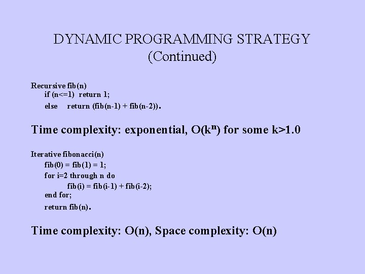
DYNAMIC PROGRAMMING STRATEGY (Continued) Recursive fib(n) if (n<=1) return 1; else return (fib(n-1) + fib(n-2)). Time complexity: exponential, O(kn) for some k>1. 0 Iterative fibonacci(n) fib(0) = fib(1) = 1; for i=2 through n do fib(i) = fib(i-1) + fib(i-2); end for; return fib(n). Time complexity: O(n), Space complexity: O(n)

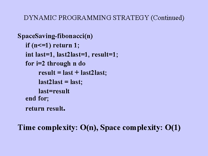
DYNAMIC PROGRAMMING STRATEGY (Continued) Space. Saving-fibonacci(n) if (n<=1) return 1; int last=1, last 2 last=1, result=1; for i=2 through n do result = last + last 2 last; last 2 last = last; last=result end for; return result. Time complexity: O(n), Space complexity: O(1)

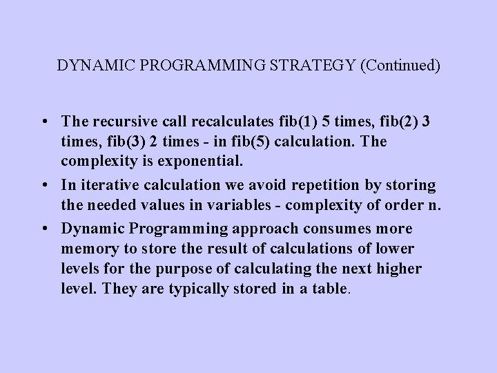
DYNAMIC PROGRAMMING STRATEGY (Continued) • The recursive call recalculates fib(1) 5 times, fib(2) 3 times, fib(3) 2 times - in fib(5) calculation. The complexity is exponential. • In iterative calculation we avoid repetition by storing the needed values in variables - complexity of order n. • Dynamic Programming approach consumes more memory to store the result of calculations of lower levels for the purpose of calculating the next higher level. They are typically stored in a table.

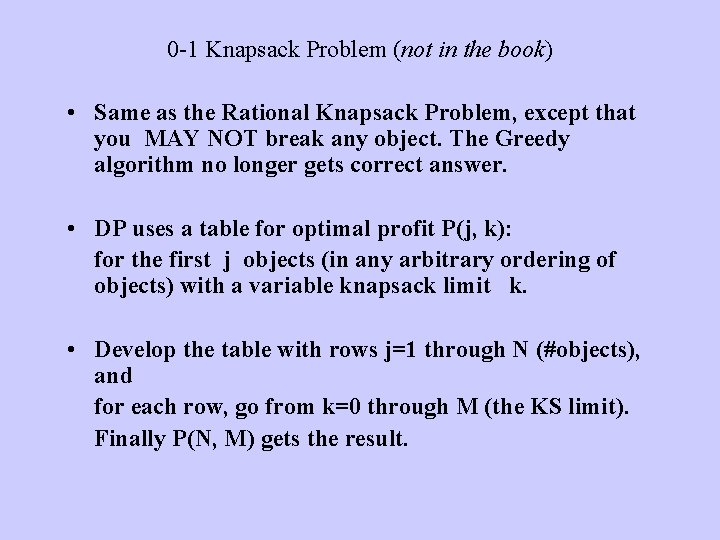
0 -1 Knapsack Problem (not in the book) • Same as the Rational Knapsack Problem, except that you MAY NOT break any object. The Greedy algorithm no longer gets correct answer. • DP uses a table for optimal profit P(j, k): for the first j objects (in any arbitrary ordering of objects) with a variable knapsack limit k. • Develop the table with rows j=1 through N (#objects), and for each row, go from k=0 through M (the KS limit). Finally P(N, M) gets the result.

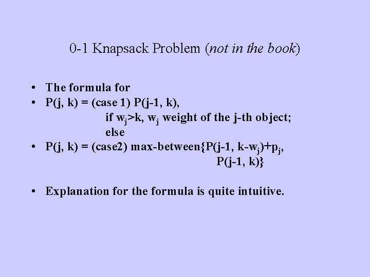
0 -1 Knapsack Problem (not in the book) • The formula for • P(j, k) = (case 1) P(j-1, k), if wj>k, wj weight of the j-th object; else • P(j, k) = (case 2) max-between{P(j-1, k-wj)+pj, P(j-1, k)} • Explanation for the formula is quite intuitive.

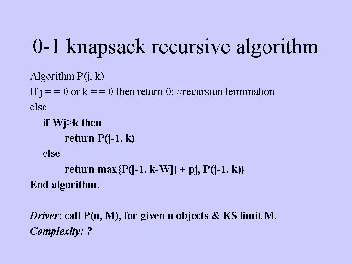
0 -1 knapsack recursive algorithm Algorithm P(j, k) If j = = 0 or k = = 0 then return 0; //recursion termination else if Wj>k then return P(j-1, k) else return max{P(j-1, k-Wj) + pj, P(j-1, k)} End algorithm. Driver: call P(n, M), for given n objects & KS limit M. Complexity: ?

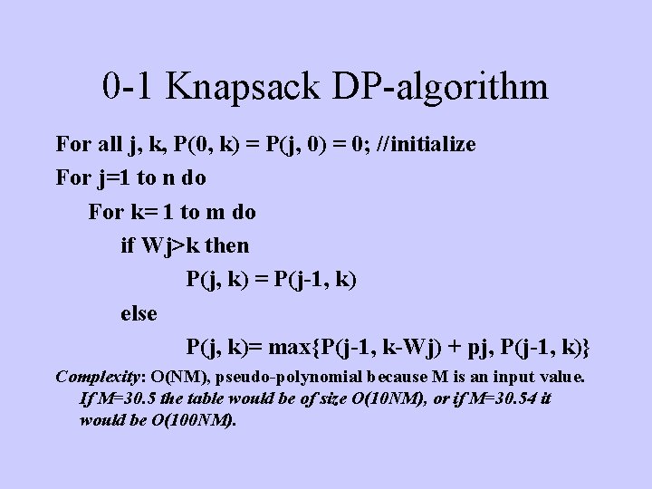
0 -1 Knapsack DP-algorithm For all j, k, P(0, k) = P(j, 0) = 0; //initialize For j=1 to n do For k= 1 to m do if Wj>k then P(j, k) = P(j-1, k) else P(j, k)= max{P(j-1, k-Wj) + pj, P(j-1, k)} Complexity: O(NM), pseudo-polynomial because M is an input value. If M=30. 5 the table would be of size O(10 NM), or if M=30. 54 it would be O(100 NM).

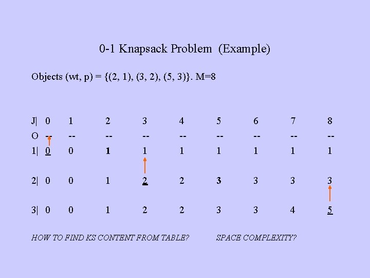
0 -1 Knapsack Problem (Example) Objects (wt, p) = {(2, 1), (3, 2), (5, 3)}. M=8 J| 0 O -1| 0 1 -0 2 -1 3 -1 4 -1 5 -1 6 -1 7 -1 8 -1 2| 0 0 1 2 2 3 3 3| 0 0 1 2 2 3 3 4 5 HOW TO FIND KS CONTENT FROM TABLE? SPACE COMPLEXITY?

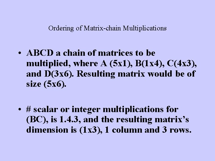
Ordering of Matrix-chain Multiplications • ABCD a chain of matrices to be multiplied, where A (5 x 1), B(1 x 4), C(4 x 3), and D(3 x 6). Resulting matrix would be of size (5 x 6). • # scalar or integer multiplications for (BC), is 1. 4. 3, and the resulting matrix’s dimension is (1 x 3), 1 column and 3 rows.

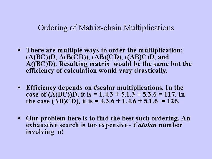
Ordering of Matrix-chain Multiplications • There are multiple ways to order the multiplication: (A(BC))D, A(B(CD)), (AB)(CD), ((AB)C)D, and A((BC)D). Resulting matrix would be the same but the efficiency of calculation would vary drastically. • Efficiency depends on #scalar multiplications. In the case of (A(BC))D, it is = 1. 4. 3 + 5. 1. 3 + 5. 3. 6 = 117. In the case (AB)CD), it is = 4. 3. 6 + 1. 4. 6 + 5. 1. 6 = 126. • Our problem here is to find the best such ordering. An exhaustive search is too expensive - Catalan number involving n!

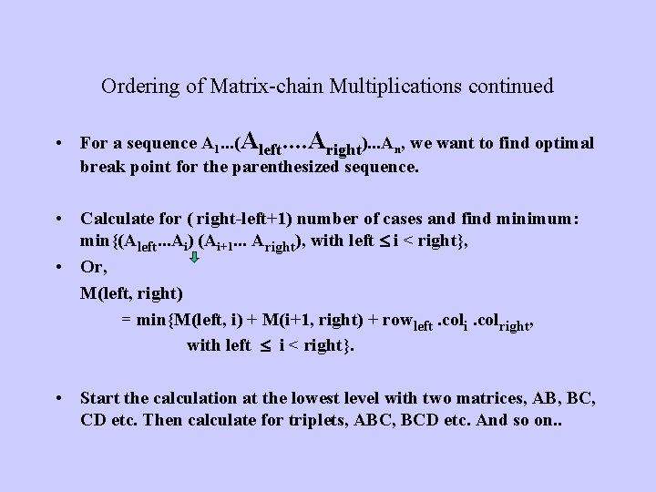
Ordering of Matrix-chain Multiplications continued • For a sequence A 1. . . (Aleft. . Aright). . . An, we want to find optimal break point for the parenthesized sequence. • Calculate for ( right-left+1) number of cases and find minimum: min{(Aleft. . . Ai) (Ai+1. . . Aright), with left i < right}, • Or, M(left, right) = min{M(left, i) + M(i+1, right) + rowleft. coli. colright, with left i < right}. • Start the calculation at the lowest level with two matrices, AB, BC, CD etc. Then calculate for triplets, ABC, BCD etc. And so on. .

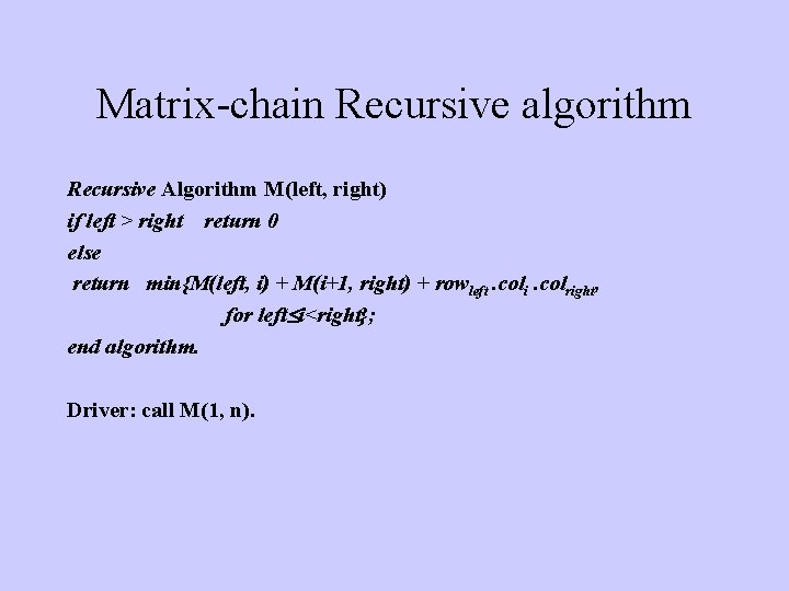
Matrix-chain Recursive algorithm Recursive Algorithm M(left, right) if left > right return 0 else return min{M(left, i) + M(i+1, right) + rowleft. coli. colright, for left i<right}; end algorithm. Driver: call M(1, n).

Matrix-chain DP-algorithm for all 1 j<i n do M[i][j] = 0; //lower triangle 0 for size = 1 to n do // size of subsequence for l =1 to n-size+1 do r = left+size-1; //move along diagonal M[l][r] = infinity; //minimizer for i = l to r do x = M(l, i) + M(i+1, r) + rowleft. coli. colright; if x < min then M(l, r) = x // Complexity?

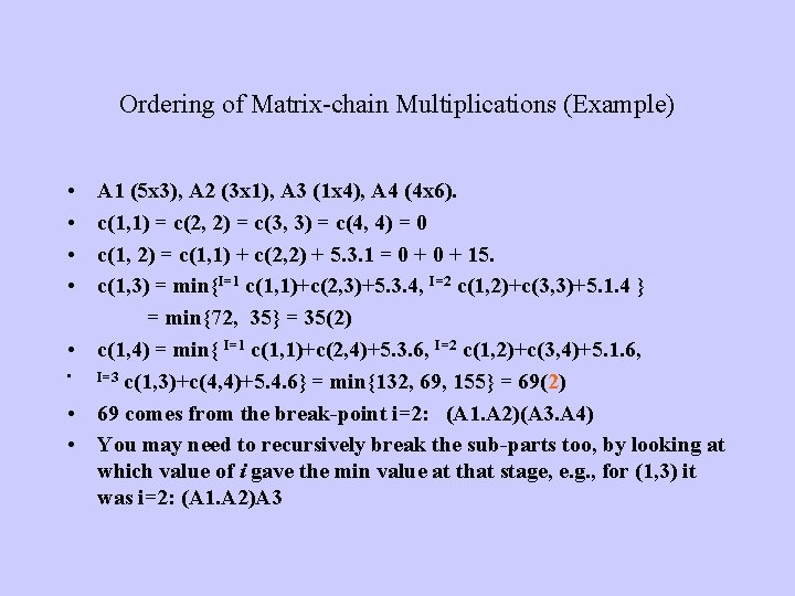
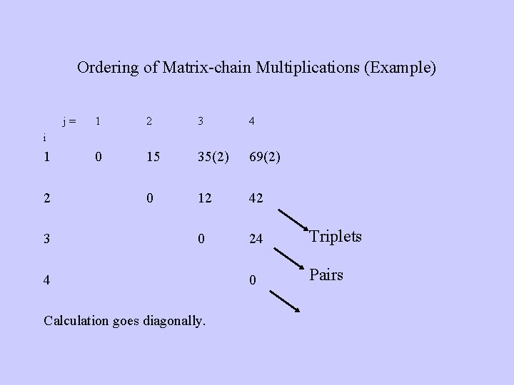
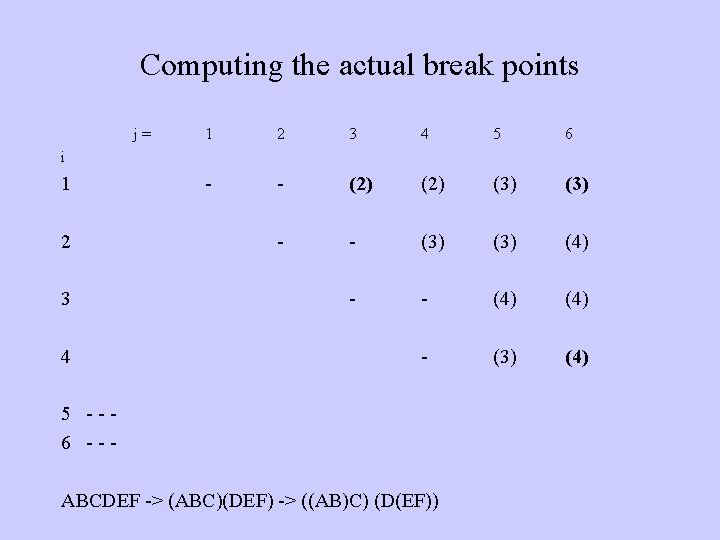
Ordering of Matrix-chain Multiplications (Example) • • A 1 (5 x 3), A 2 (3 x 1), A 3 (1 x 4), A 4 (4 x 6). c(1, 1) = c(2, 2) = c(3, 3) = c(4, 4) = 0 c(1, 2) = c(1, 1) + c(2, 2) + 5. 3. 1 = 0 + 15. c(1, 3) = min{I=1 c(1, 1)+c(2, 3)+5. 3. 4, I=2 c(1, 2)+c(3, 3)+5. 1. 4 } = min{72, 35} = 35(2) • c(1, 4) = min{ I=1 c(1, 1)+c(2, 4)+5. 3. 6, I=2 c(1, 2)+c(3, 4)+5. 1. 6, • I=3 c(1, 3)+c(4, 4)+5. 4. 6} = min{132, 69, 155} = 69(2) • 69 comes from the break-point i=2: (A 1. A 2)(A 3. A 4) • You may need to recursively break the sub-parts too, by looking at which value of i gave the min value at that stage, e. g. , for (1, 3) it was i=2: (A 1. A 2)A 3

Ordering of Matrix-chain Multiplications (Example) j= 1 2 3 4 0 15 35(2) 69(2) 0 12 42 0 24 Triplets 0 Pairs i 1 2 3 4 Calculation goes diagonally.

Computing the actual break points j= 1 2 3 4 5 6 - - (2) (3) - - (3) (4) - - (4) - (3) (4) i 1 2 3 4 5 --6 --- ABCDEF -> (ABC)(DEF) -> ((AB)C) (D(EF))

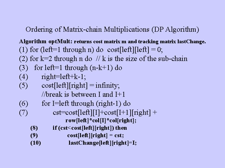
Ordering of Matrix-chain Multiplications (DP Algorithm) Algorithm opt. Mult: returns cost matrix m and tracking matrix last. Change. (1) for (left=1 through n) do cost[left] = 0; (2) for k=2 through n do // k is the size of the sub-chain (3) for left=1 through (n-k+1) do (4) right=left+k-1; (5) cost[left][right] = infinity; //break is between I and I+1 (6) for I=left through (right-1) do (7) cst=cost[left][I]+cost[I+1][right] + (8) (9) (10) row[left]*col[I]*col[right]; if (cst<cost[left][right]) then cost[left][right] = cst; last. Change[left][right]=I;

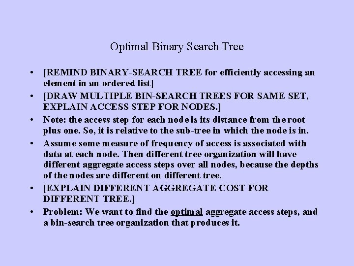
Optimal Binary Search Tree • [REMIND BINARY-SEARCH TREE for efficiently accessing an element in an ordered list] • [DRAW MULTIPLE BIN-SEARCH TREES FOR SAME SET, EXPLAIN ACCESS STEP FOR NODES. ] • Note: the access step for each node is its distance from the root plus one. So, it is relative to the sub-tree in which the node is in. • Assume some measure of frequency of access is associated with data at each node. Then different tree organization will have different aggregate access steps over all nodes, because the depths of the nodes are different on different tree. • [EXPLAIN DIFFERENT AGGREGATE COST FOR DIFFERENT TREE. ] • Problem: We want to find the optimal aggregate access steps, and a bin-search tree organization that produces it.

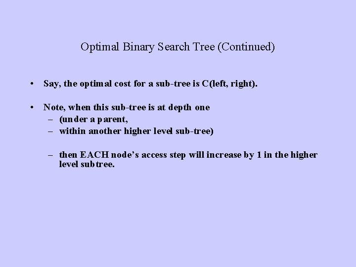
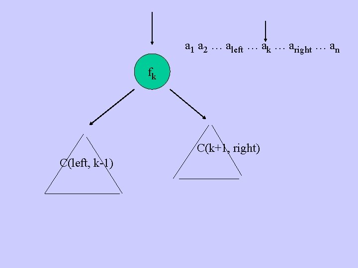
Optimal Binary Search Tree (Continued) • Say, the optimal cost for a sub-tree is C(left, right). • Note, when this sub-tree is at depth one – (under a parent, – within another higher level sub-tree) – then EACH node’s access step will increase by 1 in the higher level subtree.

a 1 a 2 … aleft … ak … aright … an fk C(k+1, right) C(left, k-1)

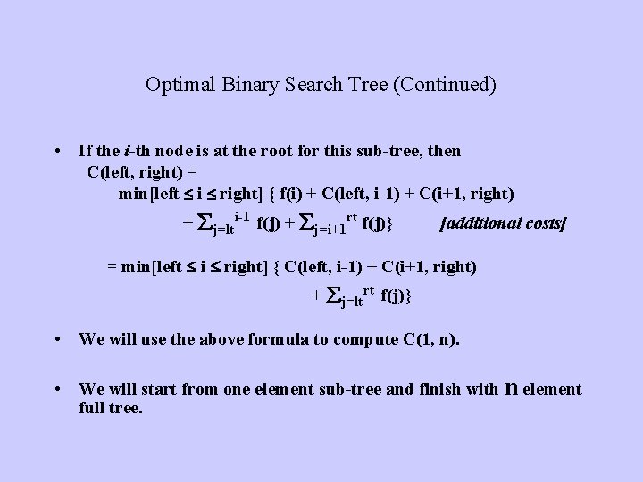
Optimal Binary Search Tree (Continued) • If the i-th node is at the root for this sub-tree, then C(left, right) = min[left i right] { f(i) + C(left, i-1) + C(i+1, right) + j=lti-1 f(j) + j=i+1 rt f(j)} [additional costs] = min[left i right] { C(left, i-1) + C(i+1, right) + j=ltrt f(j)} • We will use the above formula to compute C(1, n). • We will start from one element sub-tree and finish with n element full tree.

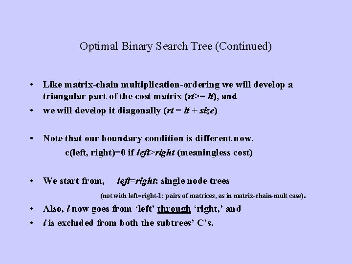
Optimal Binary Search Tree (Continued) • Like matrix-chain multiplication-ordering we will develop a triangular part of the cost matrix (rt>= lt), and • we will develop it diagonally (rt = lt + size) • Note that our boundary condition is different now, c(left, right)=0 if left>right (meaningless cost) • We start from, left=right: single node trees (not with left=right-1: pairs of matrices, as in matrix-chain-mult case). • Also, i now goes from ‘left’ through ‘right, ’ and • i is excluded from both the subtrees’ C’s.

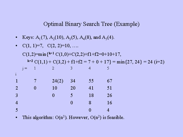
Optimal Binary Search Tree (Example) • Keys: A 1(7), A 2(10), A 3(5), A 4(8), and A 5(4). • C(1, 1)=7, C(2, 2)=10, …. C(1, 2)=min{k=1 C(1, 0)+C(2, 2)+f 1+f 2=0+10+17, k=2 C(1, 1) + C(3, 2) + f 1+f 2 = 7 + 0 + 17} = min{27, 24} = 24 (i=2) j= 1 2 3 4 5 i 1 7 24(2) 34 55 67 2 0 10 20 41 51 3 0 5 18 26 4 0 8 16 5 0 4 • This algorithm: O(n 3). However, O(n 2) is feasible.

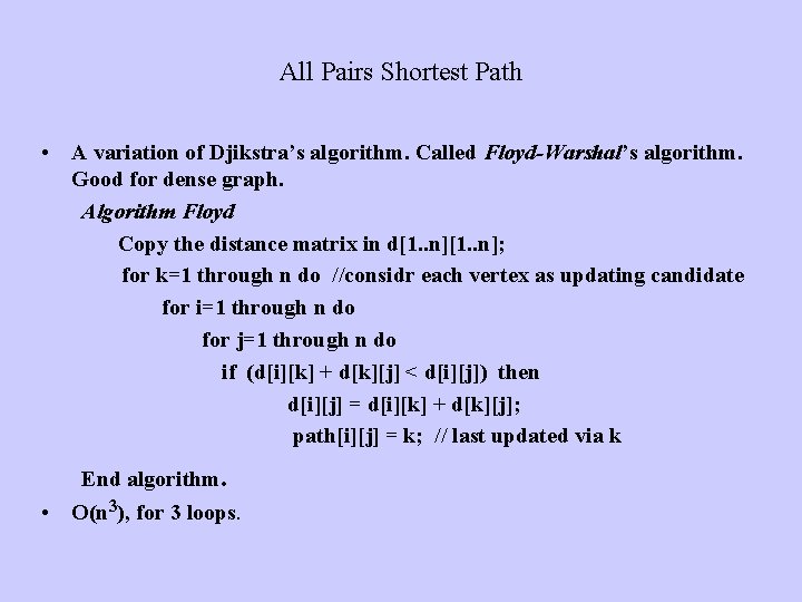
All Pairs Shortest Path • A variation of Djikstra’s algorithm. Called Floyd-Warshal’s algorithm. Good for dense graph. Algorithm Floyd Copy the distance matrix in d[1. . n]; for k=1 through n do //considr each vertex as updating candidate for i=1 through n do for j=1 through n do if (d[i][k] + d[k][j] < d[i][j]) then d[i][j] = d[i][k] + d[k][j]; path[i][j] = k; // last updated via k End algorithm. • O(n 3), for 3 loops.

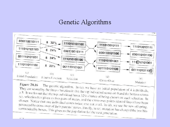
Randomized Algorithms • Quick. Sort with randomly picked up pivot is an example. • The internal working of the algorithm is never same even for the same input. Randomized algorithms may have different output for same input. • Sensitive to the embedded random number generating algorithms. Computers work with pseudo-random number generators, dependent on the key, fed at the initiation of a generator. Typically clock digits (least significant ones) are used as a key. • There are powerful randomized algorithms that can nondeterministically solve some problems more efficiently. Examples: Genetic Algorithms, or GSAT. Often these algorithms do not guarantee any solution, or are “incomplete” algorithms!

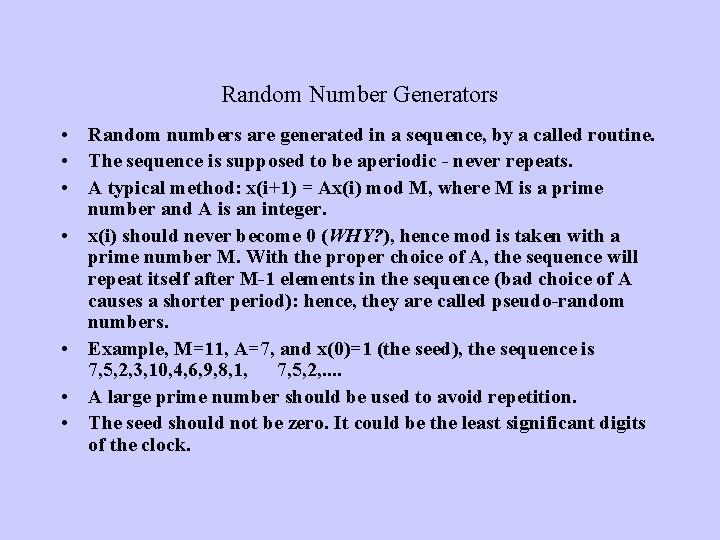
Random Number Generators • Random numbers are generated in a sequence, by a called routine. • The sequence is supposed to be aperiodic - never repeats. • A typical method: x(i+1) = Ax(i) mod M, where M is a prime number and A is an integer. • x(i) should never become 0 (WHY? ), hence mod is taken with a prime number M. With the proper choice of A, the sequence will repeat itself after M-1 elements in the sequence (bad choice of A causes a shorter period): hence, they are called pseudo-random numbers. • Example, M=11, A=7, and x(0)=1 (the seed), the sequence is 7, 5, 2, 3, 10, 4, 6, 9, 8, 1, 7, 5, 2, . . • A large prime number should be used to avoid repetition. • The seed should not be zero. It could be the least significant digits of the clock.

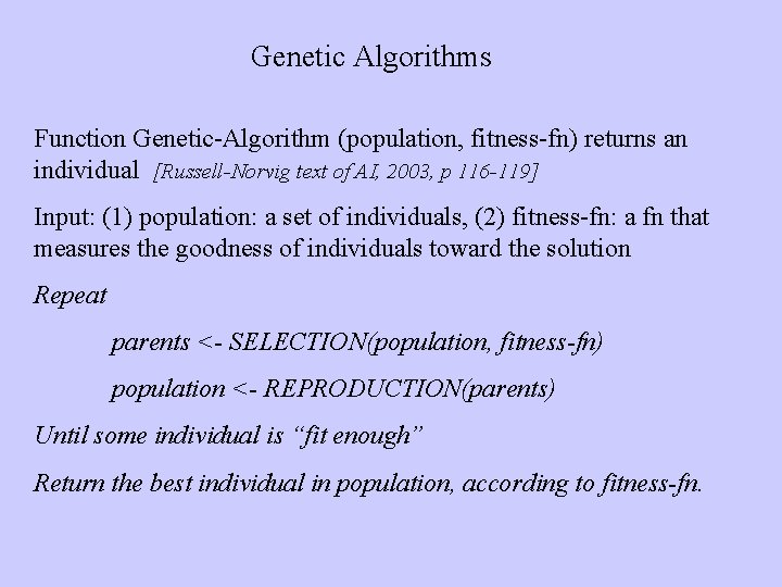
Genetic Algorithms Function Genetic-Algorithm (population, fitness-fn) returns an individual [Russell-Norvig text of AI, 2003, p 116 -119] Input: (1) population: a set of individuals, (2) fitness-fn: a fn that measures the goodness of individuals toward the solution Repeat parents <- SELECTION(population, fitness-fn) population <- REPRODUCTION(parents) Until some individual is “fit enough” Return the best individual in population, according to fitness-fn.

Genetic Algorithms

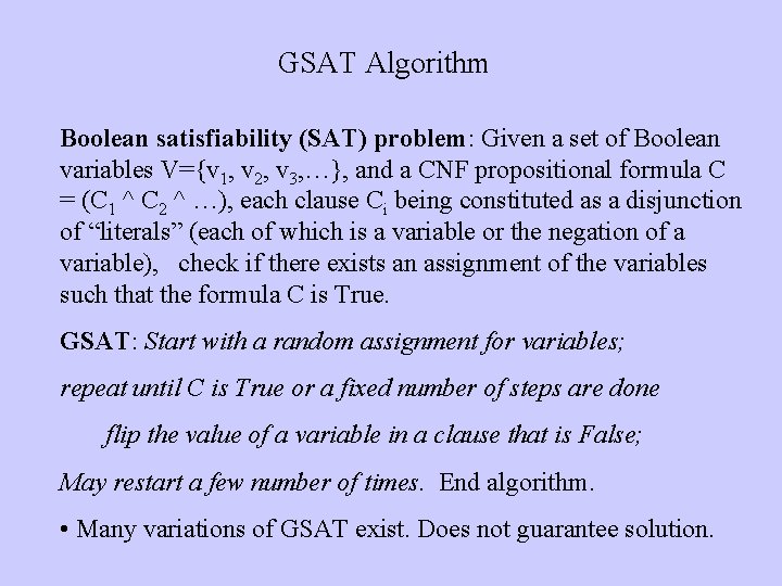
GSAT Algorithm Boolean satisfiability (SAT) problem: Given a set of Boolean variables V={v 1, v 2, v 3, …}, and a CNF propositional formula C = (C 1 ^ C 2 ^ …), each clause Ci being constituted as a disjunction of “literals” (each of which is a variable or the negation of a variable), check if there exists an assignment of the variables such that the formula C is True. GSAT: Start with a random assignment for variables; repeat until C is True or a fixed number of steps are done flip the value of a variable in a clause that is False; May restart a few number of times. End algorithm. • Many variations of GSAT exist. Does not guarantee solution.

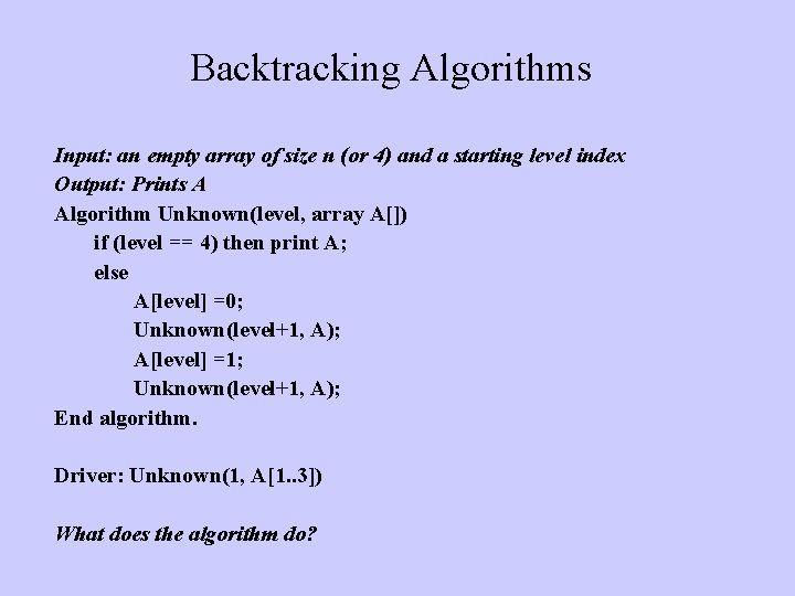
Backtracking Algorithms Input: an empty array of size n (or 4) and a starting level index Output: Prints A Algorithm Unknown(level, array A[]) if (level == 4) then print A; else A[level] =0; Unknown(level+1, A); A[level] =1; Unknown(level+1, A); End algorithm. Driver: Unknown(1, A[1. . 3]) What does the algorithm do?

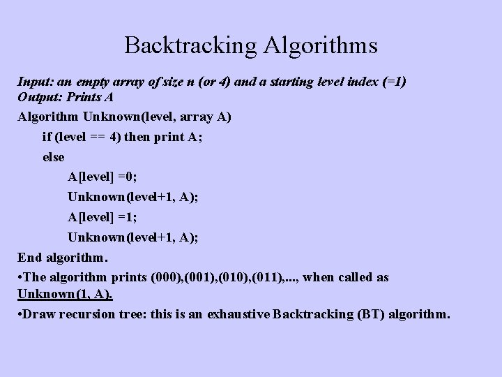
Backtracking Algorithms Input: an empty array of size n (or 4) and a starting level index (=1) Output: Prints A Algorithm Unknown(level, array A) if (level == 4) then print A; else A[level] =0; Unknown(level+1, A); A[level] =1; Unknown(level+1, A); End algorithm. • The algorithm prints (000), (001), (010), (011), . . . , when called as Unknown(1, A). • Draw recursion tree: this is an exhaustive Backtracking (BT) algorithm.

BT: 0 -1 Knapsack Problem Input: Set of n objects (w[i], p[i]), and knapsack limit=M Output: Total profits for all possible subsets Algorithm BTKS(level, array A) if (level = = n+1) then total_profit = i(A[i]*P[i]); else A[level] =0; // level-th object excluded from the bag BTKS(level+1, A); A[level] =1; // the object is included BTKS(level+1, A); End algorithm. Driver: {Global opt. P=0; Global opt. A=null; BTKS(1, A)}

BT: 0 -1 Knapsack Problem Input: Set of n objects (w[i], p[i]), and knapsack limit=M Output: Optimum profit over all possible subsets weighing <=M Algorithm BTKS(level, array A) if (level = = n+1) then total_profit = i(A[i]*P[i]); if total_profit is > opt. P then // optimizing opt. P = total_profit; opt. A = A; else A[level] =0; // level-th object excluded from the bag BTKS(level+1, A); A[level] =1; // the object is included if (total_wt M) then // constraint checking BTKS(level+1, A); End algorithm. Driver: {Global var opt. P=0; Global var opt. A=null; BTKS(1, A)}

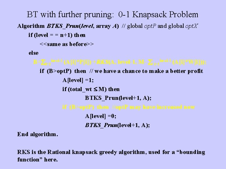
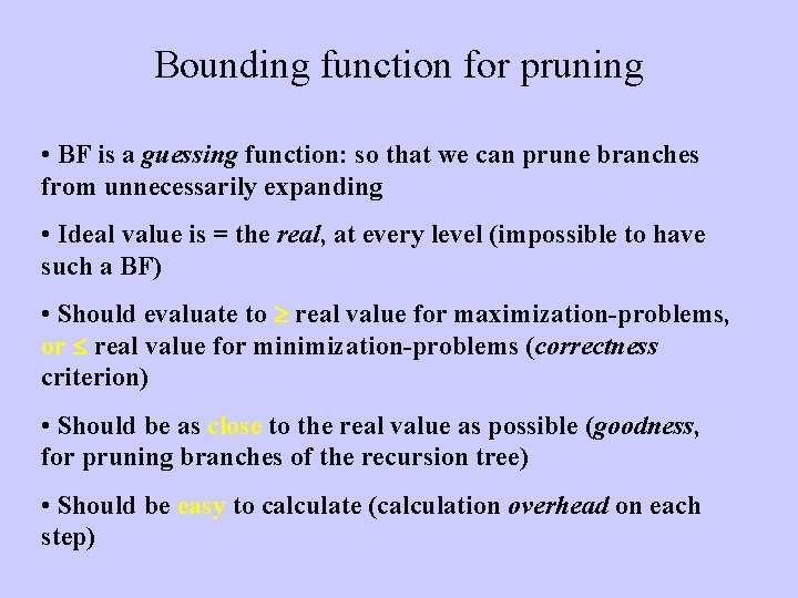
BT with further pruning: 0 -1 Knapsack Problem Algorithm BTKS_Prun(level, array A) // global opt. P and global opt. X if (level = = n+1) then <<same as before>> else B= i=1 level-1 (A[i]*P[i]) +RKS(A, level-1, M- i=1 level-1 (A[i]*W[i])); if (B>opt. P) then // we have a chance to make a better profit A[level] =1; if (total_wt M) then BTKS_Prun(level+1, A); if (B>opt. P) then //opt. P may have increased now A[level] =0; BTKS_Prun(level+1, A); End algorithm. RKS is the Rational knapsack greedy algorithm, used for a “bounding function” here.

Bounding function for pruning • BF is a guessing function: so that we can prune branches from unnecessarily expanding • Ideal value is = the real, at every level (impossible to have such a BF) • Should evaluate to real value for maximization-problems, or real value for minimization-problems (correctness criterion) • Should be as close to the real value as possible (goodness, for pruning branches of the recursion tree) • Should be easy to calculate (calculation overhead on each step)

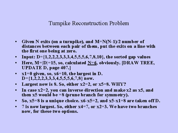
Turnpike Reconstruction Problem • Given N exits (on a turnpike), and M=N(N-1)/2 number of distances between each pair of them, put the exits on a line with the first one being at zero. • Input: D={1, 2, 2, 2, 3, 3, 3, 4, 5, 5, 5, 6, 7, 8, 10}, the sorted gap values • Here, M=|D|=15, so, calculated N=6, obviously. [DRAW TREE, UPDATE D, page 407. ] • x 1=0 given, so, x 6=10, the largest in D. D={1, 2, 2, 2, 3, 3, 3, 4, 5, 5, 5, 6, 7, 8} now. • Largest now is 8. So, either x 2=2, or x 5=8. WHY? • In case x 2=2, you can inverse direction and make x 2 as x 5, and then x 5 would be =8 (prune branch for symmetry). • So, x 5=8 is a unique choice. x 6 -x 5=2, and x 5 -x 1=8 are taken off D. • 7 is now largest. So, either x 4=7, or x 2=3. We have two branches now, for these two options.

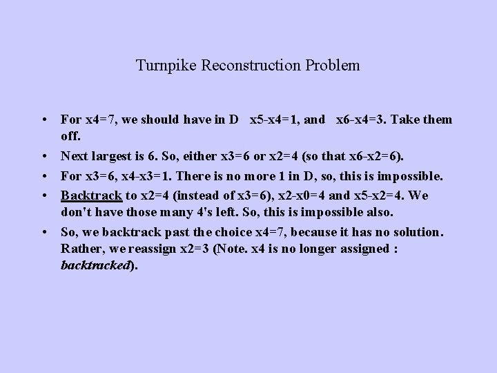
Turnpike Reconstruction Problem • For x 4=7, we should have in D x 5 -x 4=1, and x 6 -x 4=3. Take them off. • Next largest is 6. So, either x 3=6 or x 2=4 (so that x 6 -x 2=6). • For x 3=6, x 4 -x 3=1. There is no more 1 in D, so, this is impossible. • Backtrack to x 2=4 (instead of x 3=6), x 2 -x 0=4 and x 5 -x 2=4. We don't have those many 4's left. So, this is impossible also. • So, we backtrack past the choice x 4=7, because it has no solution. Rather, we reassign x 2=3 (Note. x 4 is no longer assigned : backtracked).

Turnpike Reconstruction Problem • • • For x 2=3, we take off 3, 5, 7 from D. Thus, D={1, 2, 2, 3, 3, 4, 5, 5, 6} Now, either x 4=6 or x 3=4. For x 3=4, we need two 4’s for x 3 -x 0, and x 5 -x 3. BT to x 4=6, D={1, 2, 3, 5, 5}. There is only one choice left now, i. e. , x 3=5, which fits all the values in D. • The algorithm terminates here. • Note that if backtracking leads up to the first choice and fails even there, then there is no solution (inconsistent) for the problem! • [READ ALGORITHM on p 443 -4].