Greedy algorithms Two main properties 1 Greedy choice

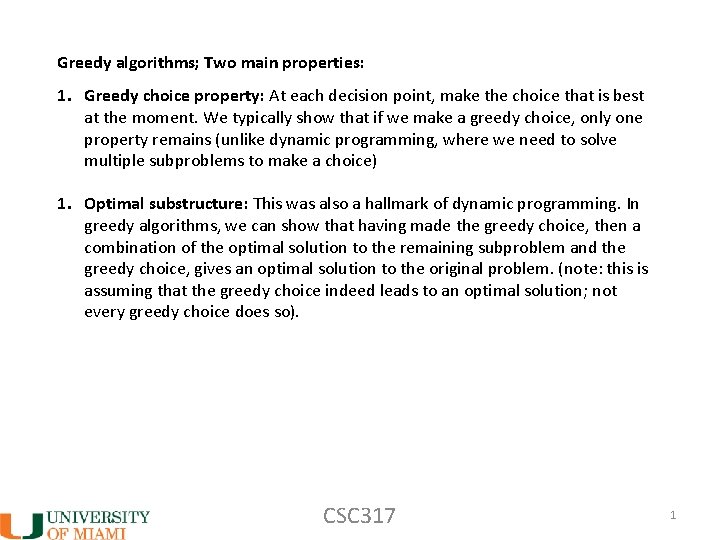
Greedy algorithms; Two main properties: 1. Greedy choice property: At each decision point, make the choice that is best at the moment. We typically show that if we make a greedy choice, only one property remains (unlike dynamic programming, where we need to solve multiple subproblems to make a choice) 1. Optimal substructure: This was also a hallmark of dynamic programming. In greedy algorithms, we can show that having made the greedy choice, then a combination of the optimal solution to the remaining subproblem and the greedy choice, gives an optimal solution to the original problem. (note: this is assuming that the greedy choice indeed leads to an optimal solution; not every greedy choice does so). CSC 317 1

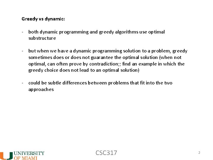
Greedy vs dynamic: - both dynamic programming and greedy algorithms use optimal substructure - but when we have a dynamic programming solution to a problem, greedy sometimes does or does not guarantee the optimal solution (when not optimal, can often prove by contradiction; ; find an example in which the greedy choice does not lead to an optimal solution) - could be subtle differences between problems that fit into the two approaches CSC 317 2

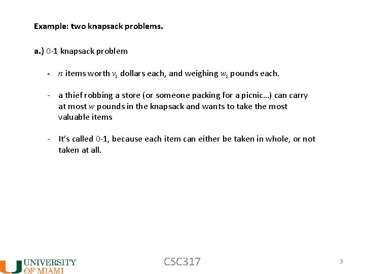
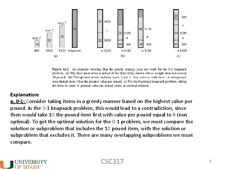
Example: two knapsack problems. a. ) 0 -1 knapsack problem - n items worth vi dollars each, and weighing wi pounds each. - a thief robbing a store (or someone packing for a picnic…) can carry at most w pounds in the knapsack and wants to take the most valuable items - It’s called 0 -1, because each item can either be taken in whole, or not taken at all. CSC 317 3

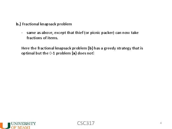
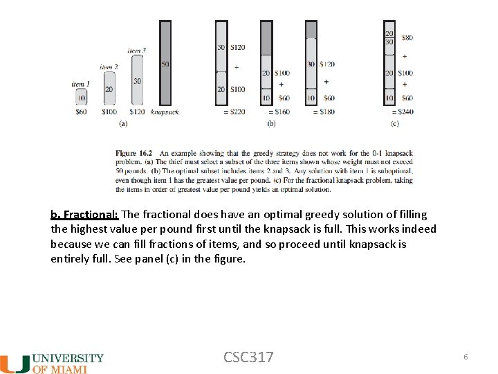
b. ) Fractional knapsack problem - same as above, except that thief (or picnic packer) can now take fractions of items. Here the fractional knapsack problem (b) has a greedy strategy that is optimal but the 0 -1 problem (a) does not! CSC 317 4

Explanation: a. 0 -1: Consider taking items in a greedy manner based on the highest value per pound. In the 0 -1 knapsack problem, this would lead to a contradiction, since then would take 10 the pound item first with value per pound equal to 6 (non optimal). To get the optimal solution for the 0 -1 problem, we must compare the solution or subproblem that includes the 10 pound item, with the solution or subproblem that excludes it. There are many overlapping subproblems we must compare. CSC 317 5

b. Fractional: The fractional does have an optimal greedy solution of filling the highest value per pound first until the knapsack is full. This works indeed because we can fill fractions of items, and so proceed until knapsack is entirely full. See panel (c) in the figure. CSC 317 6

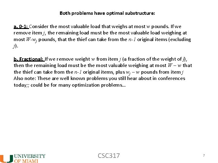
Both problems have optimal substructure: a. 0 -1: Consider the most valuable load that weighs at most w pounds. If we remove item j, the remaining load must be the most valuable load weighing at most W-wj pounds, that the thief can take from the n-1 original items (excluding j). b. Fractional: If we remove weight w from item j (a fraction of the weight of j), then the remaining load must be the most valuable weighing at most W – w that the thief can take from the n-1 original items, plus wj – w pounds from item j Also note: These are well known problems you still hear about in conferences today; ; could be for many optimization problems… CSC 317 7

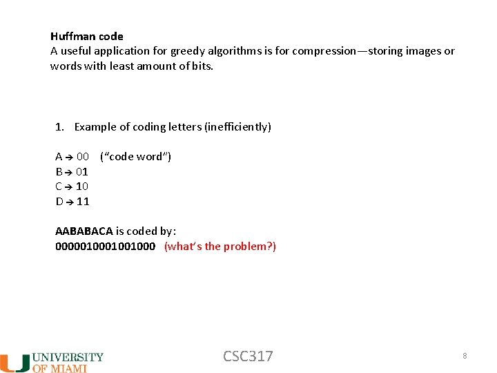
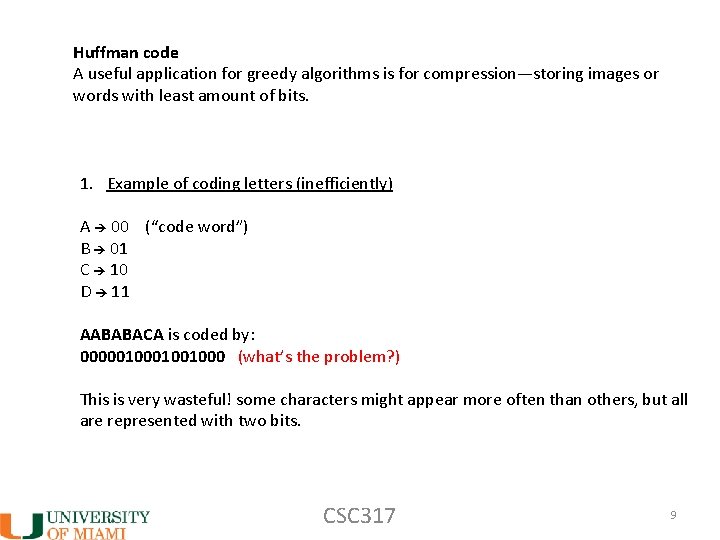
Huffman code A useful application for greedy algorithms is for compression—storing images or words with least amount of bits. 1. Example of coding letters (inefficiently) A 00 (“code word”) B 01 C 10 D 11 AABABACA is coded by: 000001001000 (what’s the problem? ) CSC 317 8

Huffman code A useful application for greedy algorithms is for compression—storing images or words with least amount of bits. 1. Example of coding letters (inefficiently) A 00 (“code word”) B 01 C 10 D 11 AABABACA is coded by: 000001001000 (what’s the problem? ) This is very wasteful! some characters might appear more often than others, but all are represented with two bits. CSC 317 9

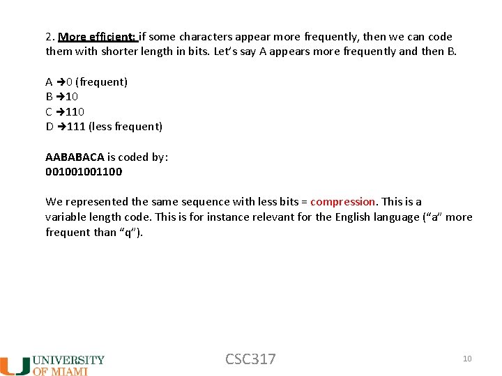
2. More efficient: if some characters appear more frequently, then we can code them with shorter length in bits. Let’s say A appears more frequently and then B. A 0 (frequent) B 10 C 110 D 111 (less frequent) AABABACA is coded by: 001001001100 We represented the same sequence with less bits = compression. This is a variable length code. This is for instance relevant for the English language (“a” more frequent than “q”). CSC 317 10

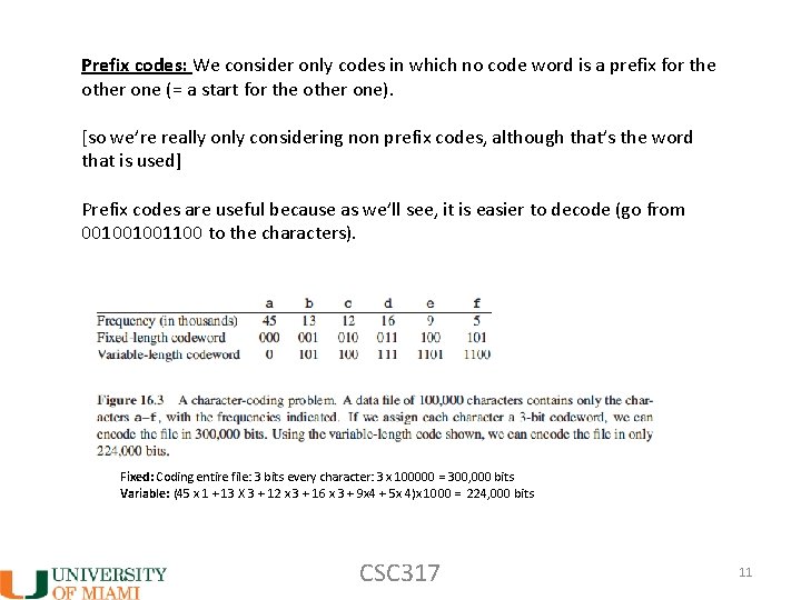
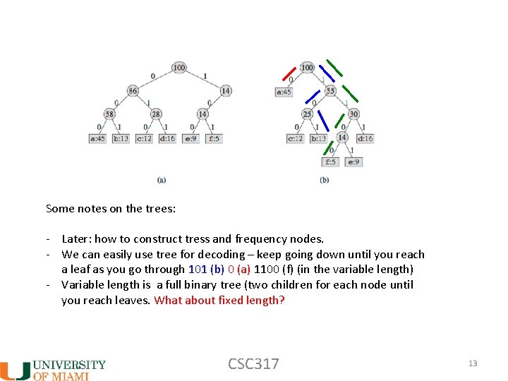
Prefix codes: We consider only codes in which no code word is a prefix for the other one (= a start for the other one). [so we’re really only considering non prefix codes, although that’s the word that is used] Prefix codes are useful because as we’ll see, it is easier to decode (go from 001001001100 to the characters). Fixed: Coding entire file: 3 bits every character: 3 x 100000 = 300, 000 bits Variable: (45 x 1 + 13 X 3 + 12 x 3 + 16 x 3 + 9 x 4 + 5 x 4)x 1000 = 224, 000 bits CSC 317 11

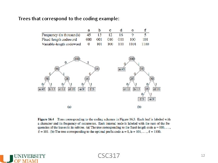
Trees that correspond to the coding example: CSC 317 12

Some notes on the trees: - Later: how to construct tress and frequency nodes. - We can easily use tree for decoding – keep going down until you reach a leaf as you go through 101 (b) 0 (a) 1100 (f) (in the variable length) - Variable length is a full binary tree (two children for each node until you reach leaves. What about fixed length? CSC 317 13

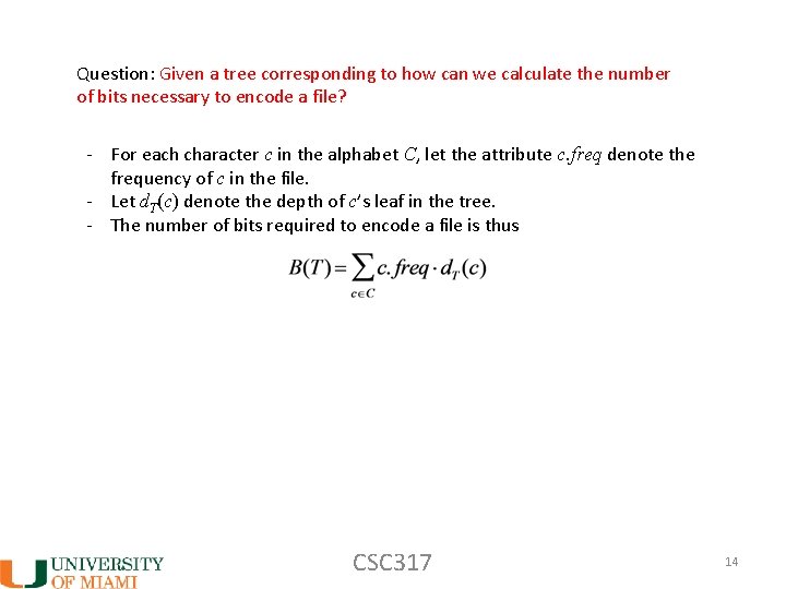
Question: Given a tree corresponding to how can we calculate the number of bits necessary to encode a file? - For each character c in the alphabet C, let the attribute c. freq denote the frequency of c in the file. - Let d. T(c) denote the depth of c’s leaf in the tree. - The number of bits required to encode a file is thus CSC 317 14

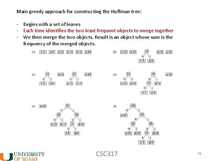
Main greedy approach for constructing the Huffman tree: - Begins with a set of leaves - Each time identifies the two least frequent objects to merge together - We then merge the two objects. Result is an object whose sum is the frequency of the merged objects. CSC 317 15

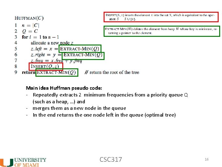
Main idea Huffman pseudo code: - Repeatedly extracts 2 minimum frequencies from a priority queue Q (such as a heap, …) and - merges them as a new node in the queue - In the end returns the one node left in the queue (optimal tree) CSC 317 16

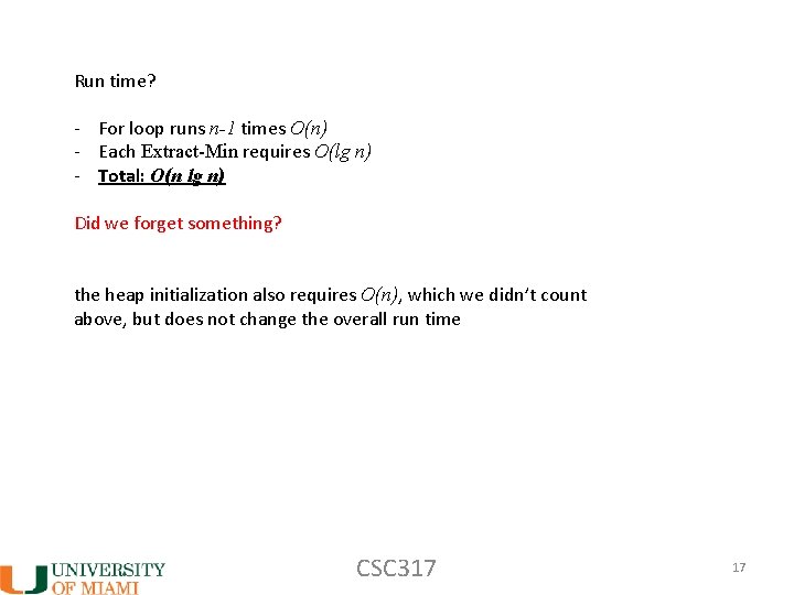
Run time? - For loop runs n-1 times O(n) - Each Extract-Min requires O(lg n) - Total: O(n lg n) Did we forget something? the heap initialization also requires O(n), which we didn’t count above, but does not change the overall run time CSC 317 17