Transform and Conquer Chapter 6 Transform and Conquer

Transform and Conquer Chapter 6

Transform and Conquer Solve problem by transforming into: a more convenient instance of the same problem (instance simplification) – presorting – Gaussian elimination

Transform and Conquer Solve problem by transforming into: a different representation of the same instance (representation change) – balanced search trees – heaps and heapsort – polynomial evaluation by Horner’s rule – Fast Fourier Transform

Transform and Conquer Solve problem by transforming into: a different problem altogether (problem reduction) – reductions to graph problems – linear programming

Instance simplification Presorting Solve instance of problem by transforming into another simpler/easier instance of the same problem

Instance simplification Presorting: Many problems involving lists are easier when list is sorted. searching computing the median (selection problem) computing the mode finding repeated elements

Selection Problem Find the kth smallest element in A[1], …A[n]. Special cases: – minimum: k = 1 – maximum: k = n – median: k = n/2 Presorting-based algorithm – sort list – return A[k]

Selection Problem Partition-based algorithm (Variable decrease & conquer): – pivot/split at A[s] using partitioning algorithm from quicksort – if s=k return A[s] – else if s<k repeat with sublist A[s+1], …A[n]. – else if s>k repeat with sublist A[1], …A[s-1]. Θ(n) average case

Notes on Selection Problem Presorting-based algorithm: Θ(n lgn) + Θ(1) = Θ(n lgn) Partition-based algorithm: Θ(n) Conclusion: Pre-sorting does NOT yield an advantage

Finding repeated elements Presorting-based algorithm: – use mergesort (or quicksort): Θ(n lgn) – scan array to find repeated adjacent elements: Θ (n ) Brute force algorithm: Θ(n 2) Conclusion: Presorting yields significant improvement

Taxonomy of Searching Algorithms Elementary searching algorithms – sequential search – binary tree search

Taxonomy of Searching Algorithms Balanced tree searching – AVL trees – red-black trees – multiway balanced trees (2 -3 trees, 2 -3 -4 trees, B trees)

Taxonomy of Searching Algorithms Hashing – separate chaining – open addressing

Balanced trees: AVL trees For every node, difference in height between left and right sub-tree is at most 1 AVL property is maintained through rotations, each time the tree becomes unbalanced lg n ≤ h ≤ 1. 4404 lg (n + 2) - 1. 3277 average: 1. 01 lg n + 0. 1 for large n

Balanced trees: AVL trees Disadvantage: needs extra storage for maintaining node balance A similar idea: red-black trees (height of subtrees is allowed to differ by up to a factor of 2)

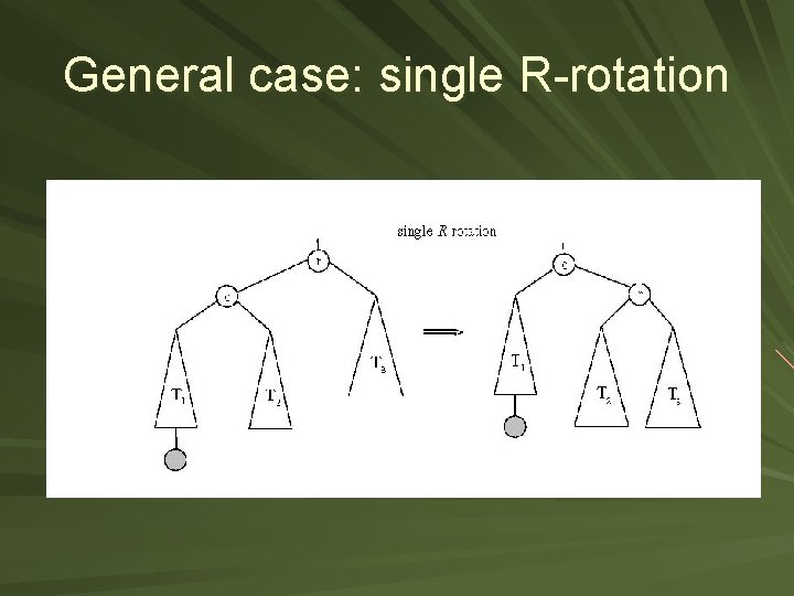
General case: single R-rotation

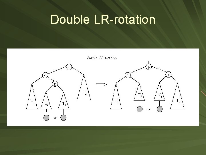
Double LR-rotation

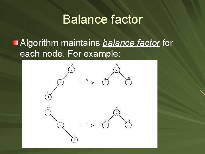
Balance factor Algorithm maintains balance factor for each node. For example:

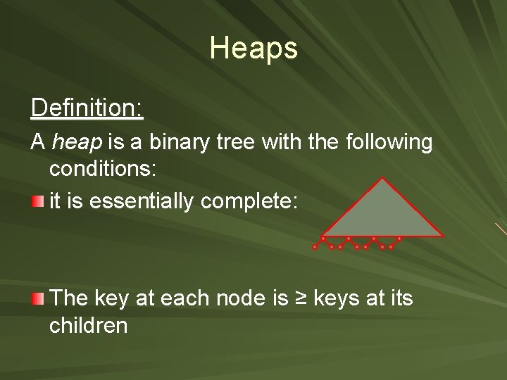
Heaps Definition: A heap is a binary tree with the following conditions: it is essentially complete: The key at each node is ≥ keys at its children

Definition implies: Given n, there exists a unique binary tree with n nodes that is essentially complete, with h= lg n The root has the largest key The subtree rooted at any node of a heap is also a heap

Heap construction Insert elements in the order given breadth -first in a binary tree Starting with the last (rightmost) parental node, fix the heap rooted at it, if it does not satisfy the heap condition: 1. exchange it with its largest child 2. fix the subtree rooted at it (now in the child’s position)

Root deletion The root of a heap can be deleted and the heap fixed up as follows: exchange the root with the last leaf compare the new root (formerly the leaf) with each of its children and, if one of them is larger than the root, exchange it with the larger of the two. continue the comparison/exchange with the children of the new root until it reaches

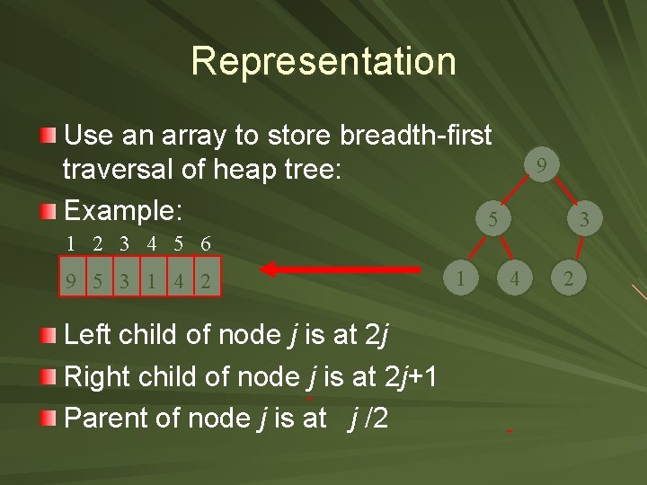
Representation Use an array to store breadth-first traversal of heap tree: Example: 5 9 3 1 2 3 4 5 6 9 5 3 1 4 2 Left child of node j is at 2 j Right child of node j is at 2 j+1 Parent of node j is at j /2 1 4 2

Priority queues A priority queue is the ADT of an ordered set with the operations: – find element with highest priority – delete element with highest priority – insert element with assigned priority Heaps are very good for implementing priority queues

Insertion of a new element Insert element at last position in heap. Compare with its parent and if it violates heap condition exchange them Continue comparing the new element with nodes up the tree until the heap condition is satisfied

Bottom-up vs. Top-down heap construction Top down: Heaps can be constructed by successively inserting elements into an (initially) empty heap Bottom-up: Put everything in and then fix it Which one is better?