More Algorithms Greedy Algorithm Dynamic Programming Algorithm tsaiwnCSIE

補充– More Algorithms Greedy Algorithm, Dynamic Programming Algorithm 蔡文能 tsaiwn@CSIE. NCTU. EDU. TW 2021/12/27 Reference: 計概課本 DP Algorithm-1

Agenda • Software Efficiency--Complexity of an Algorithm • Knapsack problem • Greedy Algorithm • Making Change problem • Knapsack problem • Dynamic Programming (DP) • DP vs. Divide-and-Conquer • Greedy vs. Dynamic Programming 2021/12/27 Reference: 計概課本 DP Algorithm-2

Software Efficiency – Time Complexity • Measured as number of instructions executed • notation for efficiency classes – O( ? ) – Q(? ) • Best, worst, and average case 2021/12/27 Reference: 計概課本 DP Algorithm-3

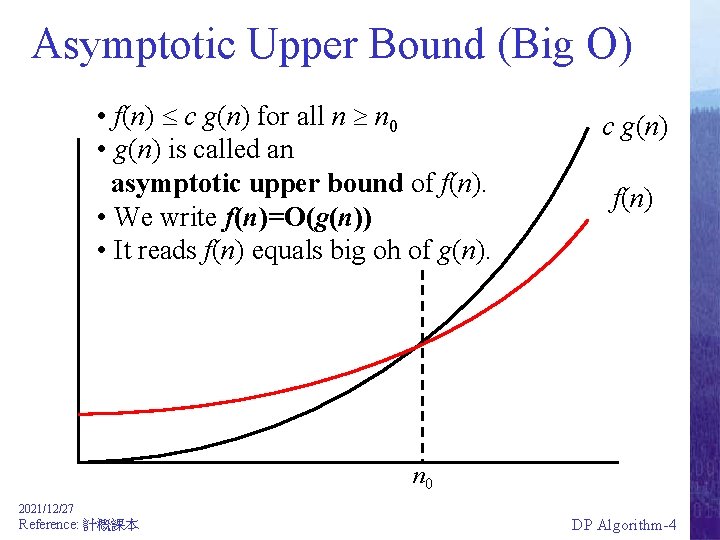
Asymptotic Upper Bound (Big O) • f(n) c g(n) for all n n 0 • g(n) is called an asymptotic upper bound of f(n). • We write f(n)=O(g(n)) • It reads f(n) equals big oh of g(n). c g(n) f(n) n 0 2021/12/27 Reference: 計概課本 DP Algorithm-4

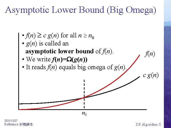
Asymptotic Lower Bound (Big Omega) • f(n) c g(n) for all n n 0 • g(n) is called an asymptotic lower bound of f(n). • We write f(n)= (g(n)) • It reads f(n) equals big omega of g(n). f(n) c g(n) n 0 2021/12/27 Reference: 計概課本 DP Algorithm-5

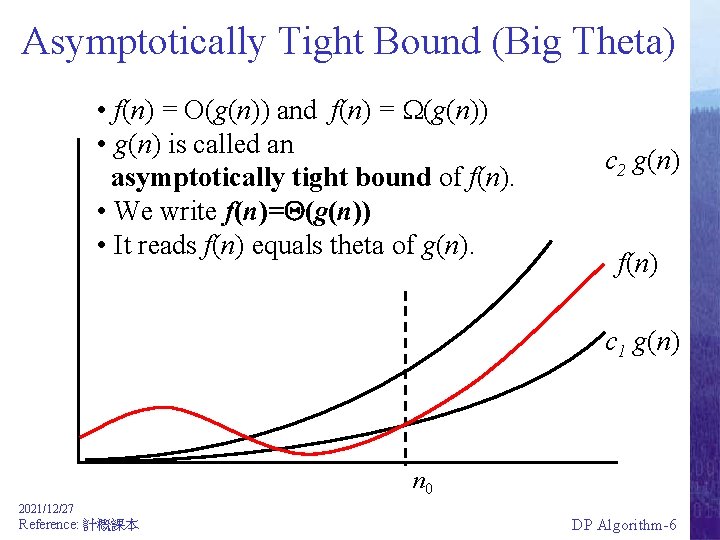
Asymptotically Tight Bound (Big Theta) • f(n) = O(g(n)) and f(n) = (g(n)) • g(n) is called an asymptotically tight bound of f(n). • We write f(n)= (g(n)) • It reads f(n) equals theta of g(n). c 2 g(n) f(n) c 1 g(n) n 0 2021/12/27 Reference: 計概課本 DP Algorithm-6

Algorithm types • Algorithm types we will consider include: – Simple recursive algorithms – Backtracking algorithms – Greedy algorithms – Divide and conquer algorithms – Dynamic programming algorithms – Branch and bound algorithms – Brute force algorithms – Randomized algorithms 2021/12/27 Reference: 計概課本 DP Algorithm-7

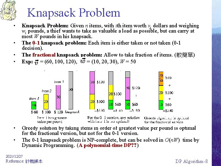
Knapsack Problem • • • Knapsack Problem: Given n items, with item worth vi dollars and weighing wi pounds, a thief wants to take as valuable a load as possible, but can carry at most W pounds in his knapsack. The 0 -1 knapsack problem: Each item is either taken or not taken (0 -1 decision). The fractional knapsack problem: Allow to take fraction of items. (較簡單) Exp: = (60, 100, 120), = (10, 20, 30), W = 50 Greedy solution by taking items in order of greatest value per pound is optimal for the fractional version, but not for the 0 -1 version. The 0 -1 knapsack problem is NP-complete, but can be solved in O(n. W) time by Dynamic Programming. (A polynomial-time DP? ? ) 2021/12/27 Reference: 計概課本 DP Algorithm-8

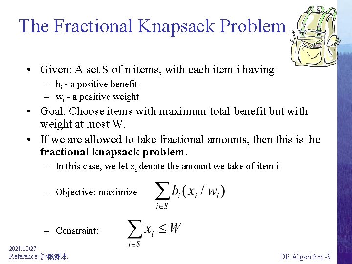
The Fractional Knapsack Problem • Given: A set S of n items, with each item i having – bi - a positive benefit – wi - a positive weight • Goal: Choose items with maximum total benefit but with weight at most W. • If we are allowed to take fractional amounts, then this is the fractional knapsack problem. – In this case, we let xi denote the amount we take of item i – Objective: maximize – Constraint: 2021/12/27 Reference: 計概課本 DP Algorithm-9

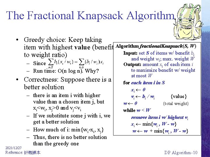
The Fractional Knapsack Algorithm • Greedy choice: Keep taking item with highest value (benefit Algorithm fractional. Knapsack(S, W) Input: set S of items w/ benefit bi to weight ratio) and weight w ; max. weight W – Since – Run time: O(n log n). Why? • Correctness: Suppose there is a better solution 2021/12/27 – there is an item i with higher value than a chosen item j, but xi<wi, xj>0 and vj<vi – If we substitute some j with i, we get a better solution – How much of i: min{wi-xi, xj} – Thus, there is no better solution than the greedy one Reference: 計概課本 i Output: amount xi of each item i to maximize benefit w/ weight at most W for each item i in S xi 0 vi bi / wi {value} w 0 {total weight} while w < W remove item i w/ highest vi xi min{wi , W - w} w w + min{wi , W - w} DP Algorithm-10

0 -1 Knapsack problem (1/5) • Given a knapsack with maximum capacity W, and a set S consisting of n items • Each item i has some weight wi and benefit value bi (all wi , bi and W are integer values) • Problem: How to pack the knapsack to achieve maximum total value of packed items? 2021/12/27 Reference: 計概課本 DP Algorithm-11

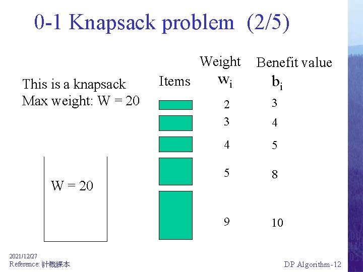
0 -1 Knapsack problem (2/5) Weight This is a knapsack Max weight: W = 20 Items wi Benefit value bi 2 3 3 4 5 5 8 9 10 4 2021/12/27 Reference: 計概課本 DP Algorithm-12

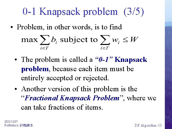
0 -1 Knapsack problem (3/5) • Problem, in other words, is to find • The problem is called a “ 0 -1” Knapsack problem, because each item must be entirely accepted or rejected. • Another version of this problem is the “Fractional Knapsack Problem”, where we can take fractions of items. 2021/12/27 Reference: 計概課本 DP Algorithm-13

0 -1 Knapsack problem (4/5) Let’s first solve this problem with a straightforward algorithm (Brute-force) ü Since there are n items, there are 2 n possible combinations of items. ü We go through all combinations and find the one with the most total value and with total weight less or equal to W. ü Running time will be O(2 n) 2021/12/27 Reference: 計概課本 DP Algorithm-14

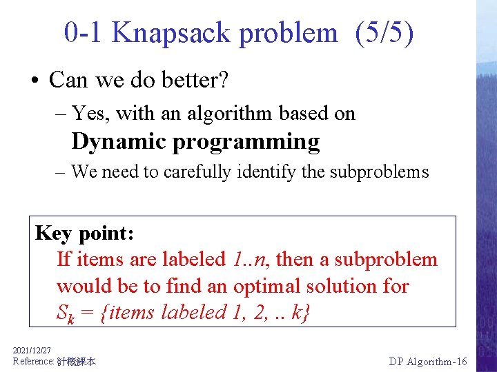
0 -1 Knapsack problem (5/5) • Can we do better? – Yes, with an algorithm based on Dynamic programming – We need to carefully identify the subproblems Key point: If items are labeled 1. . n, then a subproblem would be to find an optimal solution for Sk = {items labeled 1, 2, . . k} 2021/12/27 Reference: 計概課本 DP Algorithm-16

Algorithm types • Algorithm types we will consider include: – Simple recursive algorithms – Backtracking algorithms – Greedy algorithms – Divide and Conquer algorithms – Dynamic programming algorithms – Branch and bound algorithms – Brute force algorithms – Randomized algorithms 2021/12/27 Reference: 計概課本 DP Algorithm-17

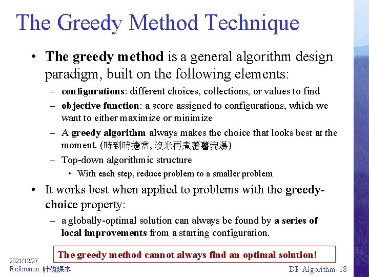
The Greedy Method Technique • The greedy method is a general algorithm design paradigm, built on the following elements: – configurations: different choices, collections, or values to find – objective function: a score assigned to configurations, which we want to either maximize or minimize – A greedy algorithm always makes the choice that looks best at the moment. (時到時擔當, 沒米再煮蕃薯塊湯) – Top-down algorithmic structure • With each step, reduce problem to a smaller problem • It works best when applied to problems with the greedychoice property: – a globally-optimal solution can always be found by a series of local improvements from a starting configuration. 2021/12/27 The greedy method cannot always find an optimal solution! Reference: 計概課本 DP Algorithm-18

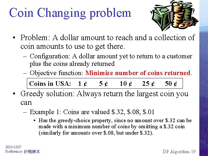
Coin Changing problem • Problem: A dollar amount to reach and a collection of coin amounts to use to get there. – Configuration: A dollar amount yet to return to a customer plus the coins already returned – Objective function: Minimize number of coins returned. Coins in USA: 1¢ 5¢ 10 ¢ 25 ¢ 50 ¢ • Greedy solution: Always return the largest coin you can – Example 1: Coins are valued $. 32, $. 08, $. 01 • Has the greedy-choice property, since no amount over $. 32 can be made with a minimum number of coins by omitting a $. 32 coin (similarly for amounts over $. 08, but under $. 32). 2021/12/27 Reference: 計概課本 DP Algorithm-19

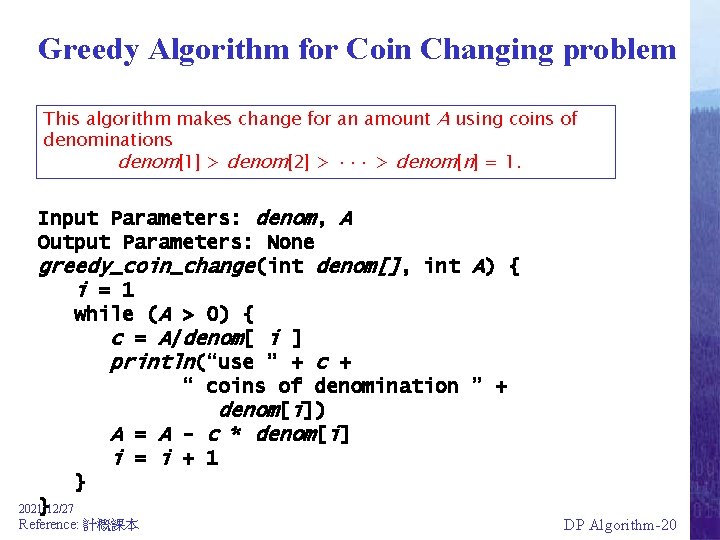
Greedy Algorithm for Coin Changing problem This algorithm makes change for an amount A using coins of denominations denom[1] > denom[2] > ··· > denom[n] = 1. Input Parameters: denom, A Output Parameters: None greedy_coin_change(int denom[], int A) { i = 1 while (A > 0) { c = A/denom[ i ] println(“use ” + c + “ coins of denomination ” + denom[i]) A = A - c * denom[i] i = i + 1 } } 2021/12/27 Reference: 計概課本 DP Algorithm-20

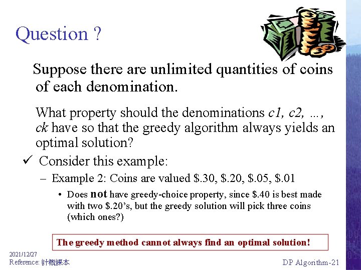
Question ? Suppose there are unlimited quantities of coins of each denomination. What property should the denominations c 1, c 2, …, ck have so that the greedy algorithm always yields an optimal solution? ü Consider this example: – Example 2: Coins are valued $. 30, $. 20, $. 05, $. 01 • Does not have greedy-choice property, since $. 40 is best made with two $. 20’s, but the greedy solution will pick three coins (which ones? ) The greedy method cannot always find an optimal solution! 2021/12/27 Reference: 計概課本 DP Algorithm-21

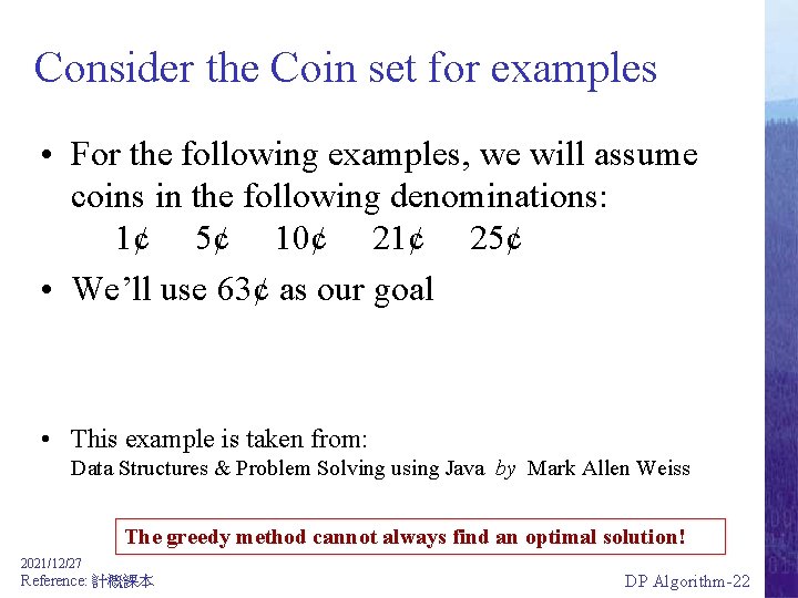
Consider the Coin set for examples • For the following examples, we will assume coins in the following denominations: 1¢ 5¢ 10¢ 21¢ 25¢ • We’ll use 63¢ as our goal • This example is taken from: Data Structures & Problem Solving using Java by Mark Allen Weiss The greedy method cannot always find an optimal solution! 2021/12/27 Reference: 計概課本 DP Algorithm-22

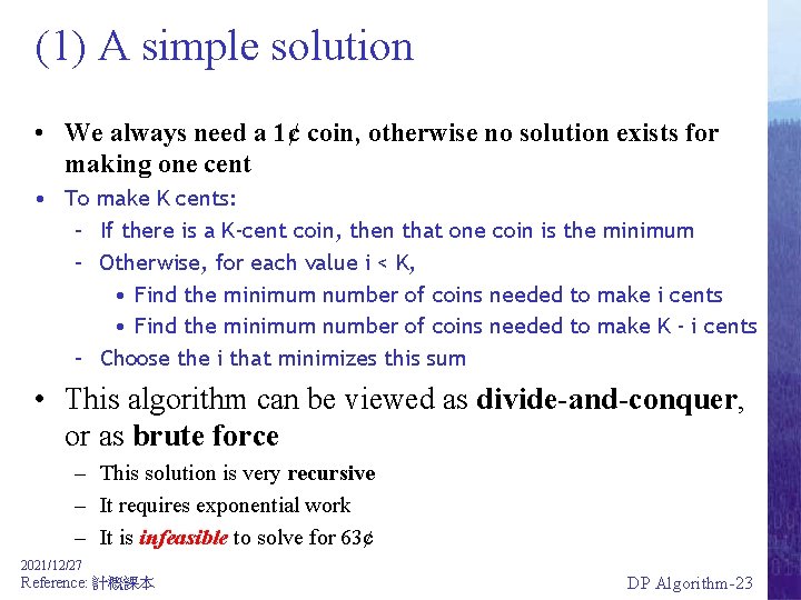
(1) A simple solution • We always need a 1¢ coin, otherwise no solution exists for making one cent • To make K cents: – If there is a K-cent coin, then that one coin is the minimum – Otherwise, for each value i < K, • Find the minimum number of coins needed to make i cents • Find the minimum number of coins needed to make K - i cents – Choose the i that minimizes this sum • This algorithm can be viewed as divide-and-conquer, or as brute force – This solution is very recursive – It requires exponential work – It is infeasible to solve for 63¢ 2021/12/27 Reference: 計概課本 DP Algorithm-23

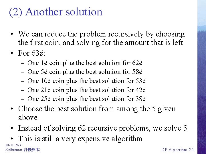
(2) Another solution • We can reduce the problem recursively by choosing the first coin, and solving for the amount that is left • For 63¢: – – – One 1¢ coin plus the best solution for 62¢ One 5¢ coin plus the best solution for 58¢ One 10¢ coin plus the best solution for 53¢ One 21¢ coin plus the best solution for 42¢ One 25¢ coin plus the best solution for 38¢ • Choose the best solution from among the 5 given above • Instead of solving 62 recursive problems, we solve 5 • This is still a very expensive algorithm 2021/12/27 Reference: 計概課本 DP Algorithm-24

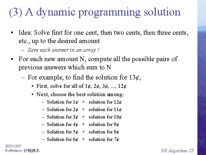
(3) A dynamic programming solution • Idea: Solve first for one cent, then two cents, then three cents, etc. , up to the desired amount – Save each answer in an array ! • For each new amount N, compute all the possible pairs of previous answers which sum to N – For example, to find the solution for 13¢, • First, solve for all of 1¢, 2¢, 3¢, . . . , 12¢ • Next, choose the best solution among: – – – Solution for 1¢ Solution for 2¢ Solution for 3¢ Solution for 4¢ Solution for 5¢ Solution for 6¢ + + + solution for 12¢ solution for 11¢ solution for 10¢ solution for 9¢ solution for 8¢ solution for 7¢ 2021/12/27 Reference: 計概課本 DP Algorithm-25

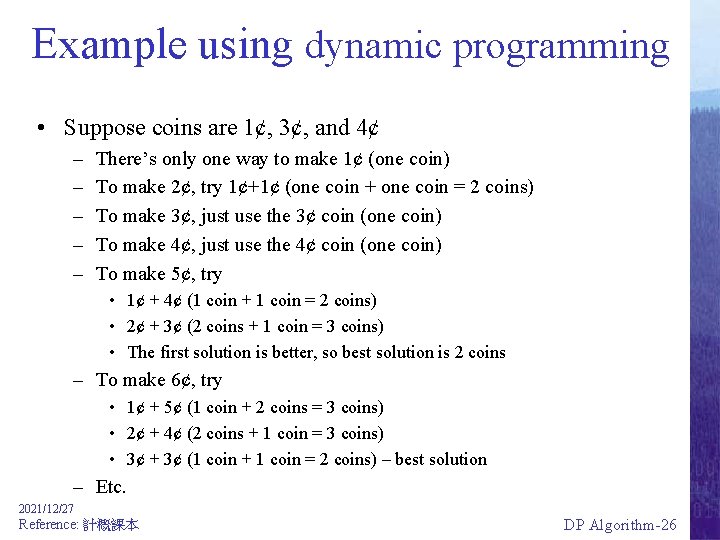
Example using dynamic programming • Suppose coins are 1¢, 3¢, and 4¢ – – – There’s only one way to make 1¢ (one coin) To make 2¢, try 1¢+1¢ (one coin + one coin = 2 coins) To make 3¢, just use the 3¢ coin (one coin) To make 4¢, just use the 4¢ coin (one coin) To make 5¢, try • 1¢ + 4¢ (1 coin + 1 coin = 2 coins) • 2¢ + 3¢ (2 coins + 1 coin = 3 coins) • The first solution is better, so best solution is 2 coins – To make 6¢, try • 1¢ + 5¢ (1 coin + 2 coins = 3 coins) • 2¢ + 4¢ (2 coins + 1 coin = 3 coins) • 3¢ + 3¢ (1 coin + 1 coin = 2 coins) – best solution – Etc. 2021/12/27 Reference: 計概課本 DP Algorithm-26

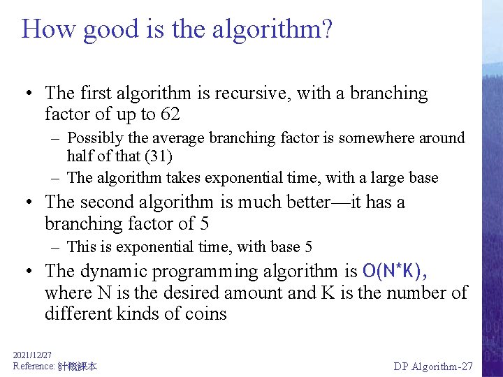
How good is the algorithm? • The first algorithm is recursive, with a branching factor of up to 62 – Possibly the average branching factor is somewhere around half of that (31) – The algorithm takes exponential time, with a large base • The second algorithm is much better—it has a branching factor of 5 – This is exponential time, with base 5 • The dynamic programming algorithm is O(N*K), where N is the desired amount and K is the number of different kinds of coins 2021/12/27 Reference: 計概課本 DP Algorithm-27

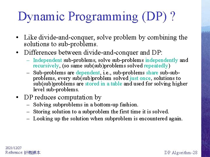
Dynamic Programming (DP) ? • Like divide-and-conquer, solve problem by combining the solutions to sub-problems. • Differences between divide-and-conquer and DP: – Independent sub-problems, solve sub-problems independently and recursively, (so same sub(sub)problems solved repeatedly) – Sub-problems are dependent, i. e. , sub-problems share sub-subproblems, every sub(sub)problem solved just once, solutions to sub(sub)problems are stored in a table and used for solving higher level sub-problems. • DP reduces computation by – Solving subproblems in a bottom-up fashion. – Storing solution to a subproblem the first time it is solved. – Looking up the solution when subproblem is encountered again. 2021/12/27 Reference: 計概課本 DP Algorithm-28

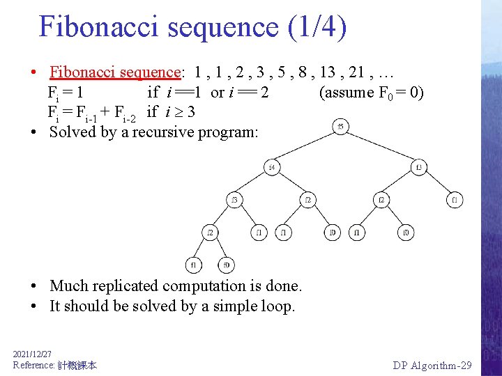
Fibonacci sequence (1/4) • Fibonacci sequence: 1 , 2 , 3 , 5 , 8 , 13 , 21 , … Fi = 1 if i ==1 or i == 2 (assume F 0 = 0) Fi = Fi-1 + Fi-2 if i 3 • Solved by a recursive program: • Much replicated computation is done. • It should be solved by a simple loop. 2021/12/27 Reference: 計概課本 DP Algorithm-29

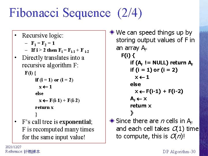
Fibonacci Sequence (2/4) • Recursive logic: – F 1 = F 2 = 1 – If i > 2 then Fi = Fi-1 + F i-2 • Directly translates into a recursive algorithm F: F(i) { if (i = 1) or (i = 2) x 1 else x F(i-1) + F(i-2) return x } • F’s call tree is exponential; F is recomputed many times for the same input value! We can speed things up by storing output values of F in an array AF F(i) { if (AF != NULL) return AF if (i = 1) or (i = 2) x 1 else x F(i-1) + F(i-2) AF x return x } Since there are n cells in AF and each cell takes O(1) time to compute, this is O(n)! 2021/12/27 Reference: 計概課本 DP Algorithm-30

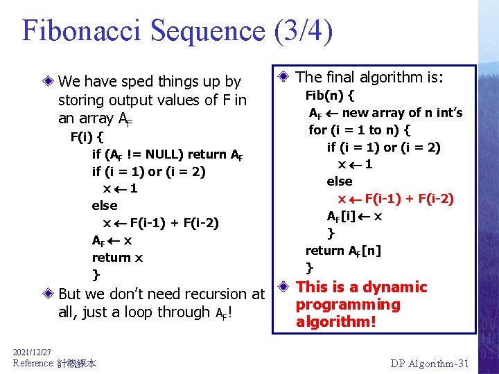
Fibonacci Sequence (3/4) We have sped things up by storing output values of F in an array AF The final algorithm is: But we don’t need recursion at all, just a loop through AF! This is a dynamic programming algorithm! F(i) { if (AF != NULL) return AF if (i = 1) or (i = 2) x 1 else x F(i-1) + F(i-2) AF x return x } Fib(n) { AF new array of n int’s for (i = 1 to n) { if (i = 1) or (i = 2) x 1 else x F(i-1) + F(i-2) AF[i] x } return AF[n] } 2021/12/27 Reference: 計概課本 DP Algorithm-31

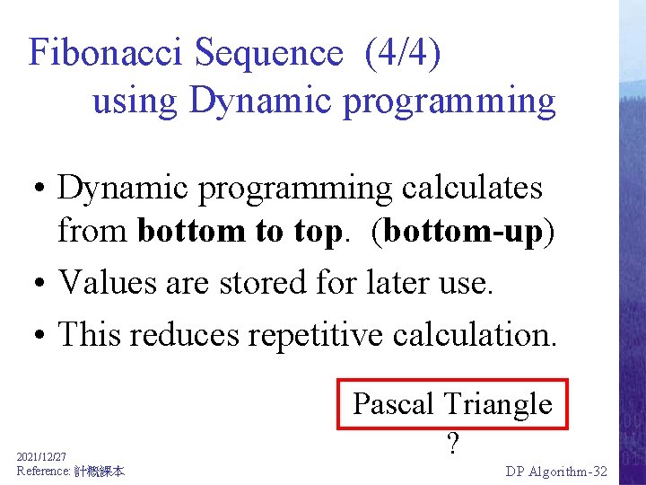
Fibonacci Sequence (4/4) using Dynamic programming • Dynamic programming calculates from bottom to top. (bottom-up) • Values are stored for later use. • This reduces repetitive calculation. 2021/12/27 Reference: 計概課本 Pascal Triangle ? DP Algorithm-32

Application domain of DP • Optimization problem: find a solution with optimal (maximum or minimum) value. • An optimal solution, not the optimal solution, since may more than one optimal solution, any one is OK. • Dynamic Programming is an algorithm design method that can be used when the solution to a problem may be viewed as the result of a sequence of decisions 2021/12/27 Reference: 計概課本 DP Algorithm-33

Typical steps of DP • Characterize the structure of an optimal solution. • Recursively define the value of an optimal solution. • Compute the value of an optimal solution in a bottom-up fashion. • Compute an optimal solution from computed/stored information. 2021/12/27 Reference: 計概課本 DP Algorithm-34

Comparison with Divide-and-Conquer • Divide-and-conquer algorithms split a problem into separate subproblems, solve the subproblems, and combine the results for a solution to the original problem – Example: Quicksort – Example: Mergesort – Example: Binary search Divide-and-Conquer 分割征服 ; 各個擊破; 拆解 • Divide-and-Conquer algorithms can be thought of as top-down algorithms • In contrast, a dynamic programming algorithm proceeds by solving small problems, then combining them to find the solution to larger problems • Dynamic programming can be thought of as bottom-up 2021/12/27 Reference: 計概課本 DP Algorithm-35

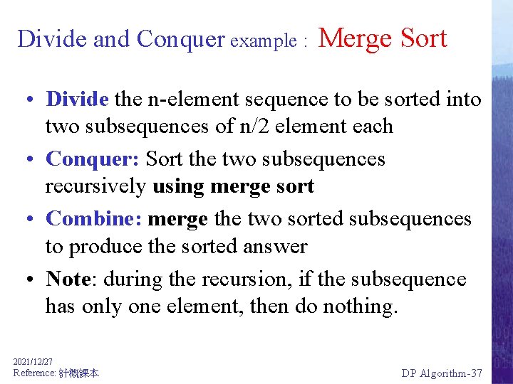
Divide and Conquer • Divide the problem into a number of sub -problems (similar to the original problem but smaller); • Conquer the sub-problems by solving them recursively (if a sub-problem is small enough, just solve it in a straightforward manner (base case). ) • Combine the solutions to the sub-problems into the solution for the original problem 2021/12/27 Reference: 計概課本 DP Algorithm-36

Divide and Conquer example : Merge Sort • Divide the n-element sequence to be sorted into two subsequences of n/2 element each • Conquer: Sort the two subsequences recursively using merge sort • Combine: merge the two sorted subsequences to produce the sorted answer • Note: during the recursion, if the subsequence has only one element, then do nothing. 2021/12/27 Reference: 計概課本 DP Algorithm-37

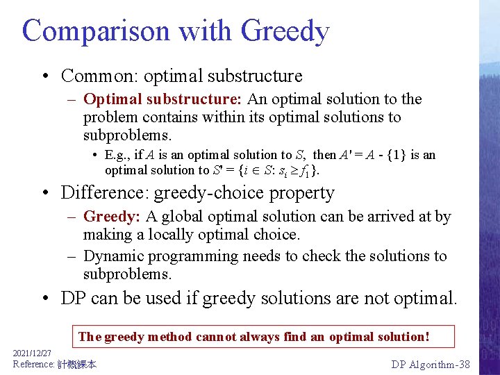
Comparison with Greedy • Common: optimal substructure – Optimal substructure: An optimal solution to the problem contains within its optimal solutions to subproblems. • E. g. , if A is an optimal solution to S, then A' = A - {1} is an optimal solution to S' = {i S: si f 1}. • Difference: greedy-choice property – Greedy: A global optimal solution can be arrived at by making a locally optimal choice. – Dynamic programming needs to check the solutions to subproblems. • DP can be used if greedy solutions are not optimal. The greedy method cannot always find an optimal solution! 2021/12/27 Reference: 計概課本 DP Algorithm-38

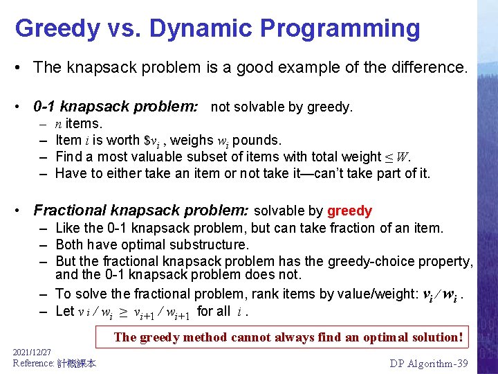
Greedy vs. Dynamic Programming • The knapsack problem is a good example of the difference. • 0 -1 knapsack problem: not solvable by greedy. – – n items. Item i is worth $vi , weighs wi pounds. Find a most valuable subset of items with total weight ≤ W. Have to either take an item or not take it—can’t take part of it. • Fractional knapsack problem: solvable by greedy – Like the 0 -1 knapsack problem, but can take fraction of an item. – Both have optimal substructure. – But the fractional knapsack problem has the greedy-choice property, and the 0 -1 knapsack problem does not. – To solve the fractional problem, rank items by value/weight: vi / wi. – Let v i / wi ≥ vi+1 / wi+1 for all i. The greedy method cannot always find an optimal solution! 2021/12/27 Reference: 計概課本 DP Algorithm-39

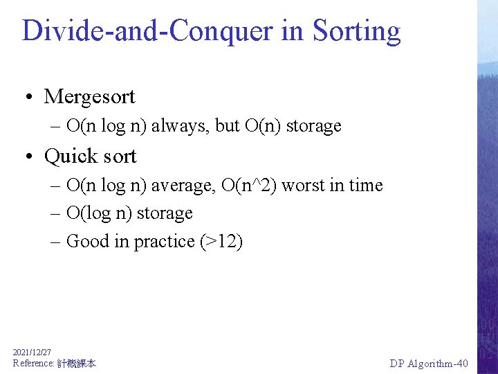
Divide-and-Conquer in Sorting • Mergesort – O(n log n) always, but O(n) storage • Quick sort – O(n log n) average, O(n^2) worst in time – O(log n) storage – Good in practice (>12) 2021/12/27 Reference: 計概課本 DP Algorithm-40

Computer Game-playing • Can computers beat humans in board games like Chess, Checkers, Go, 六子棋? • This is one of the first tasks of Artificial Intelligence (Shannon 1950) • Successes obtained in Chess (Deep Blue), Checkers, Draughts, Backgammon, Scrabble. . . 2021/12/27 Reference: 計概課本 DP Algorithm-41

Game-playing • Domain: two-player zero-sum game with perfect information (Zermelo, 1913) • Task: find best response to opponent’s moves, provided that the opponent does the same • Solution: Minimax procedure (von Neumann, 1928) 2021/12/27 Reference: 計概課本 DP Algorithm-42

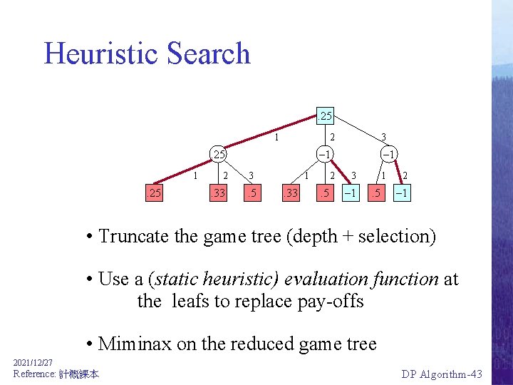
Heuristic Search. 25 1 2 . 25 1 . 25 3 – 1 2 3 . 33 . 5 1 . 33 2 . 5 – 1 3 – 1 1 . 5 2 – 1 • Truncate the game tree (depth + selection) • Use a (static heuristic) evaluation function at the leafs to replace pay-offs • Miminax on the reduced game tree 2021/12/27 Reference: 計概課本 DP Algorithm-43

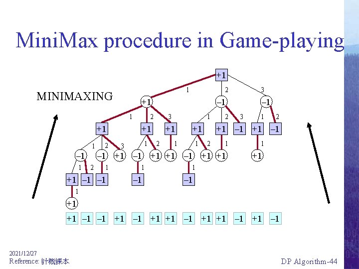
Mini. Max procedure in Game-playing +1 1 MINIMAXING +1 1 – 1 1 2 2 – 1 2 3 +1 1 3 1 +1 2 +1 1 1 2 1 +1 – 1 – 1 3 1 2 +1 – 1 2 1 – 1 +1 +1 2 3 1 +1 1 – 1 1 +1 +1 – 1 +1 +1 – 1 2021/12/27 Reference: 計概課本 DP Algorithm-44

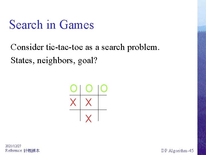
Search in Games Consider tic-tac-toe as a search problem. States, neighbors, goal? O O O X X X 2021/12/27 Reference: 計概課本 DP Algorithm-45

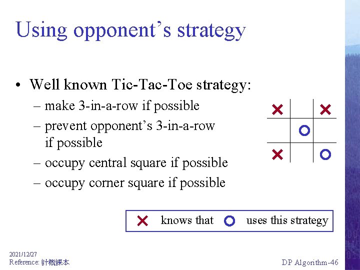
Using opponent’s strategy • Well known Tic-Tac-Toe strategy: – make 3 -in-a-row if possible – prevent opponent’s 3 -in-a-row if possible – occupy central square if possible – occupy corner square if possible knows that uses this strategy 2021/12/27 Reference: 計概課本 DP Algorithm-46

Opponent-Model search Iida, vd Herik, Uiterwijk (1993) Carmel and Markovitch (1993) • Opponent’s evaluation function is known (unilateral: the opponent uses minimax) • This is the opponent model • It is used to predict opponent’s moves • Best response is determined, using the own evaluation function 2021/12/27 Reference: 計概課本 DP Algorithm-47

Nim: Example Game n piles of sticks, ci sticks in pile i X: sizes of piles on player 1’s turn Y: sizes of piles on player 2’s turn N(s): all reductions of a pile by one or more, swapping turns G(s): all sticks gone V(s): +1 if s in X, else -1 (lose if take last stick) 2021/12/27 Reference: 計概課本 DP Algorithm-48

Heuristic Evaluation Familiar idea: Compute h(s), a value meant to correlate with the game-theoretic value of the game. After searching as deeply as possible, plug in h(s) instead of searching to leaves. 2021/12/27 Reference: 計概課本 DP Algorithm-49

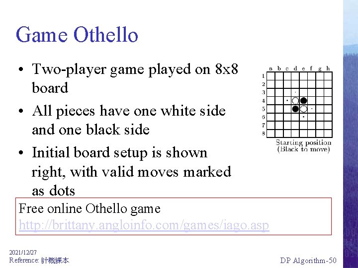
Game Othello • Two-player game played on 8 x 8 board • All pieces have one white side and one black side • Initial board setup is shown right, with valid moves marked as dots Free online Othello game http: //brittany. angloinfo. com/games/iago. asp 2021/12/27 Reference: 計概課本 DP Algorithm-50

The Evolution of Strong Othello Programs Michael Buro, 2003 • First computer Othello tournaments in 1979 • In 1980, first time a World-champion lost a game of skill against a computer • 6 -0 defeat of then human World-champion in 1997 • Michael Buro http: //www. cs. ualberta. ca/~mburo/ 2021/12/27 Reference: 計概課本 DP Algorithm-51

Evaluation Function Evolution • Mini-max search used to estimate the chance of winning for the player with current move • Construct function using features of board state that correlate with winning • Important features – Disc stability – stable discs cannot be flipped – Disc mobility – move options – Disc parity – last move opportunities for every empty board region 2021/12/27 Reference: 計概課本 DP Algorithm-52