Introduction to Algorithms Greedy Algorithms Greedy Algorithms A
![An The Optimal Substructure of the A. -S. Problem • c[i, j] : size An The Optimal Substructure of the A. -S. Problem • c[i, j] : size](https://slidetodoc.com/presentation_image_h2/72f6856312335a18a79336dc6fd98326/image-14.jpg)







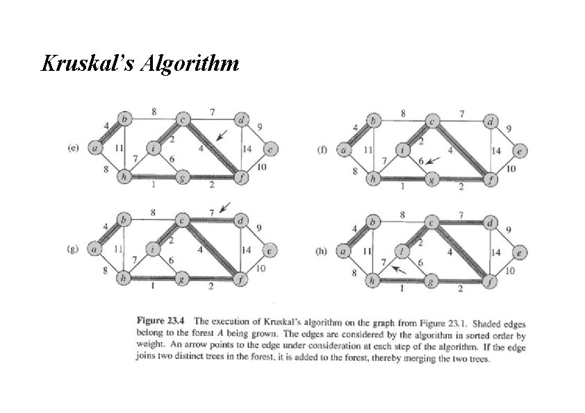
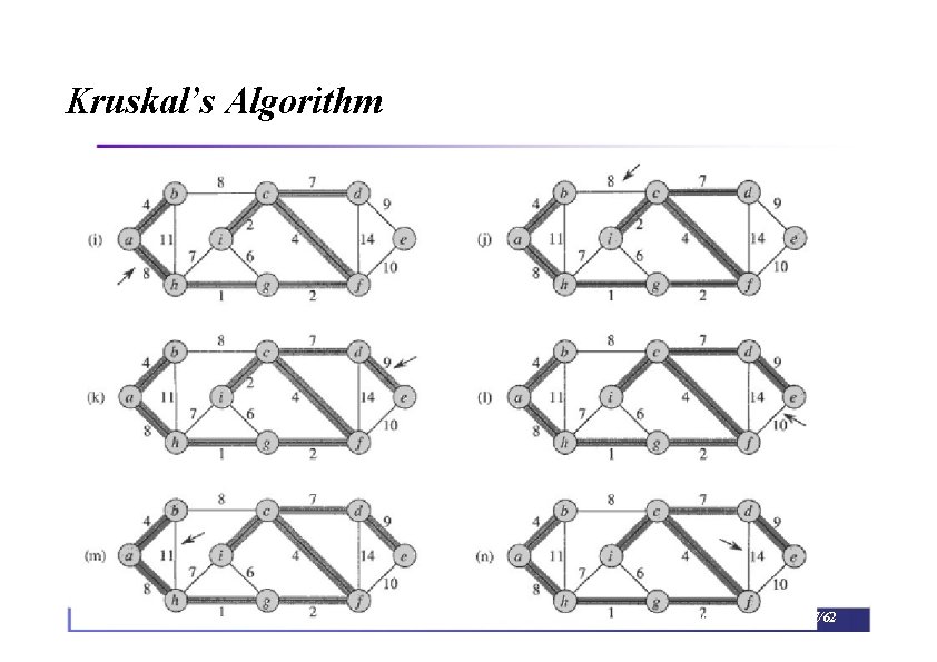
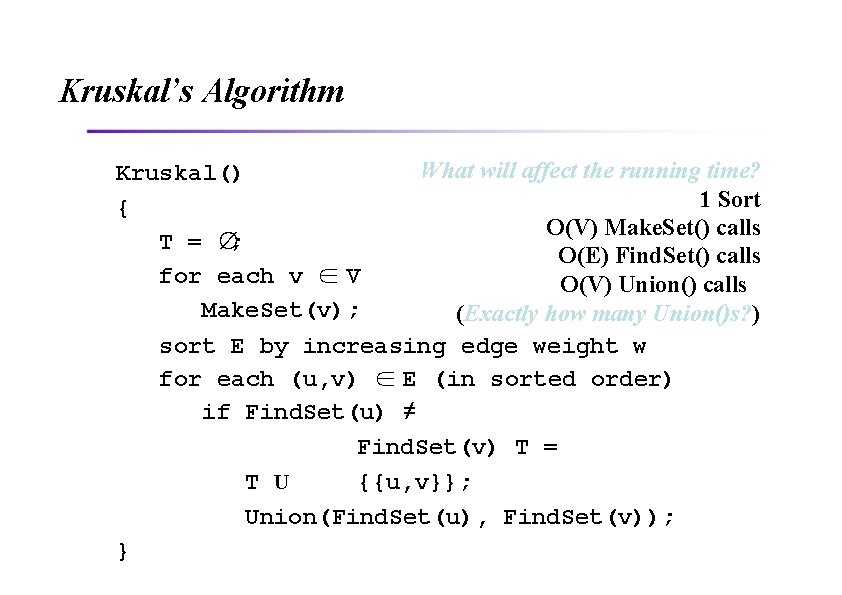
![Prim’s Algorithm MST-Prim(G, w, r) 6 Q = V[G]; 4 for each u ∈ Prim’s Algorithm MST-Prim(G, w, r) 6 Q = V[G]; 4 for each u ∈](https://slidetodoc.com/presentation_image_h2/72f6856312335a18a79336dc6fd98326/image-60.jpg)
![Prim’s Algorithm • r) Q = V[G]; 14 • П[r] = NULL; • while Prim’s Algorithm • r) Q = V[G]; 14 • П[r] = NULL; • while](https://slidetodoc.com/presentation_image_h2/72f6856312335a18a79336dc6fd98326/image-61.jpg)
![Prim’s Algorithm • r) Q = V[G]; 14 r • П[r] = NULL; • Prim’s Algorithm • r) Q = V[G]; 14 r • П[r] = NULL; •](https://slidetodoc.com/presentation_image_h2/72f6856312335a18a79336dc6fd98326/image-62.jpg)
![Prim’s Algorithm MST-Prim(G, w, r) Q = V[G]; key[u] = ∞; key[r] = 0; Prim’s Algorithm MST-Prim(G, w, r) Q = V[G]; key[u] = ∞; key[r] = 0;](https://slidetodoc.com/presentation_image_h2/72f6856312335a18a79336dc6fd98326/image-63.jpg)
![Prim’s Algorithm • r) Q = V[G]; 14 u • П[r] = NULL; • Prim’s Algorithm • r) Q = V[G]; 14 u • П[r] = NULL; •](https://slidetodoc.com/presentation_image_h2/72f6856312335a18a79336dc6fd98326/image-64.jpg)
![Prim’s Algorithm MST-Prim(G, w, r) ∞ 6 Q = V[G]; key[u] = ∞; key[r] Prim’s Algorithm MST-Prim(G, w, r) ∞ 6 Q = V[G]; key[u] = ∞; key[r]](https://slidetodoc.com/presentation_image_h2/72f6856312335a18a79336dc6fd98326/image-65.jpg)
![Prim’s Algorithm MST-Prim(G, w, r) ∞ 6 Q = V[G]; for each u ∈Q Prim’s Algorithm MST-Prim(G, w, r) ∞ 6 Q = V[G]; for each u ∈Q](https://slidetodoc.com/presentation_image_h2/72f6856312335a18a79336dc6fd98326/image-66.jpg)
![Prim’s Algorithm MST-Prim(G, w, r) ∞ 6 Q = V[G]; for each u ∈Q Prim’s Algorithm MST-Prim(G, w, r) ∞ 6 Q = V[G]; for each u ∈Q](https://slidetodoc.com/presentation_image_h2/72f6856312335a18a79336dc6fd98326/image-67.jpg)
![Prim’s Algorithm MST-Prim(G, w, r) ∞ 6 Q = V[G]; for each u ∈Q Prim’s Algorithm MST-Prim(G, w, r) ∞ 6 Q = V[G]; for each u ∈Q](https://slidetodoc.com/presentation_image_h2/72f6856312335a18a79336dc6fd98326/image-68.jpg)
![Prim’s Algorithm MST-Prim(G, w, r) ∞ 6 Q = V[G]; for each u ∈Q Prim’s Algorithm MST-Prim(G, w, r) ∞ 6 Q = V[G]; for each u ∈Q](https://slidetodoc.com/presentation_image_h2/72f6856312335a18a79336dc6fd98326/image-69.jpg)
![Prim’s Algorithm MST-Prim(G, w, r) ∞ 6 Q = V[G]; for each u ∈Q Prim’s Algorithm MST-Prim(G, w, r) ∞ 6 Q = V[G]; for each u ∈Q](https://slidetodoc.com/presentation_image_h2/72f6856312335a18a79336dc6fd98326/image-70.jpg)
![Prim’s Algorithm MST-Prim(G, w, r) ∞ 6 Q = V[G]; for each u ∈Q Prim’s Algorithm MST-Prim(G, w, r) ∞ 6 Q = V[G]; for each u ∈Q](https://slidetodoc.com/presentation_image_h2/72f6856312335a18a79336dc6fd98326/image-71.jpg)
![Prim’s Algorithm MST-Prim(G, w, r) ∞ 6 Q = V[G]; for each u ∈Q Prim’s Algorithm MST-Prim(G, w, r) ∞ 6 Q = V[G]; for each u ∈Q](https://slidetodoc.com/presentation_image_h2/72f6856312335a18a79336dc6fd98326/image-72.jpg)
![Prim’s Algorithm MST-Prim(G, w, r) ∞ 6 Q = V[G]; for each u ∈Q Prim’s Algorithm MST-Prim(G, w, r) ∞ 6 Q = V[G]; for each u ∈Q](https://slidetodoc.com/presentation_image_h2/72f6856312335a18a79336dc6fd98326/image-73.jpg)
![Prim’s Algorithm MST-Prim(G, w, r) 4 6 Q = V[G]; for each u ∈Q Prim’s Algorithm MST-Prim(G, w, r) 4 6 Q = V[G]; for each u ∈Q](https://slidetodoc.com/presentation_image_h2/72f6856312335a18a79336dc6fd98326/image-74.jpg)
![Prim’s Algorithm MST-Prim(G, w, r) 4 6 Q = V[G]; for each u ∈Q Prim’s Algorithm MST-Prim(G, w, r) 4 6 Q = V[G]; for each u ∈Q](https://slidetodoc.com/presentation_image_h2/72f6856312335a18a79336dc6fd98326/image-75.jpg)
![Prim’s Algorithm MST-Prim(G, w, r) 4 6 Q = V[G]; key[u] = ∞; key[r] Prim’s Algorithm MST-Prim(G, w, r) 4 6 Q = V[G]; key[u] = ∞; key[r]](https://slidetodoc.com/presentation_image_h2/72f6856312335a18a79336dc6fd98326/image-76.jpg)
![Prim’s Algorithm u MST-Prim(G, w, r) Q = V[G]; 4 5 5 for each Prim’s Algorithm u MST-Prim(G, w, r) Q = V[G]; 4 5 5 for each](https://slidetodoc.com/presentation_image_h2/72f6856312335a18a79336dc6fd98326/image-77.jpg)
![Prim’s Algorithm MST-Prim(G, w, r) 4 6 Q = V[G]; for each u ∈Q Prim’s Algorithm MST-Prim(G, w, r) 4 6 Q = V[G]; for each u ∈Q](https://slidetodoc.com/presentation_image_h2/72f6856312335a18a79336dc6fd98326/image-78.jpg)
![Prim’s Algorithm MST-Prim(G, w, r) 4 6 Q = V[G]; key[u] = ∞; key[r] Prim’s Algorithm MST-Prim(G, w, r) 4 6 Q = V[G]; key[u] = ∞; key[r]](https://slidetodoc.com/presentation_image_h2/72f6856312335a18a79336dc6fd98326/image-79.jpg)
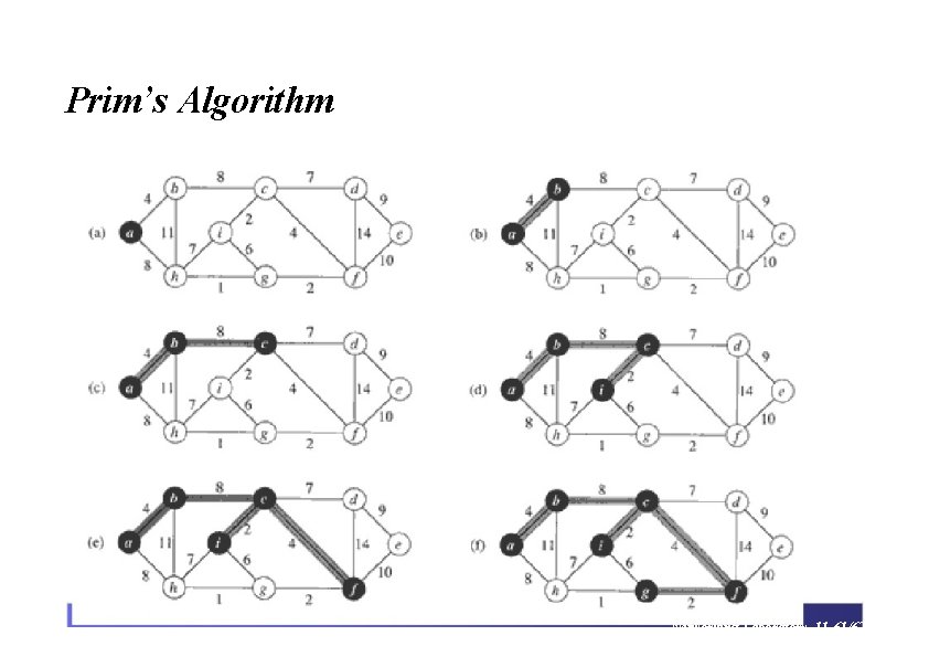
- Slides: 107

Introduction to Algorithms Greedy Algorithms

Greedy Algorithms • A greedy algorithm always makes the choice that looks best at the moment • My everyday examples • Playing cards • Invest on stocks • Choose a university • The hope • A locally optimal choice will lead to a globally optimal solution

Introduction • Similar to Dynamic Programming • It applies to Optimization Problem • When we have a choice to make, make the one that looks best right now • Make a locally optimal choice in hope of getting a globally optimal solution • Greedy algorithms don’t always yield an optimal solution, but sometimes they do • For many problems, it provides an optimal solution much more quickly than a dynamic programming approach

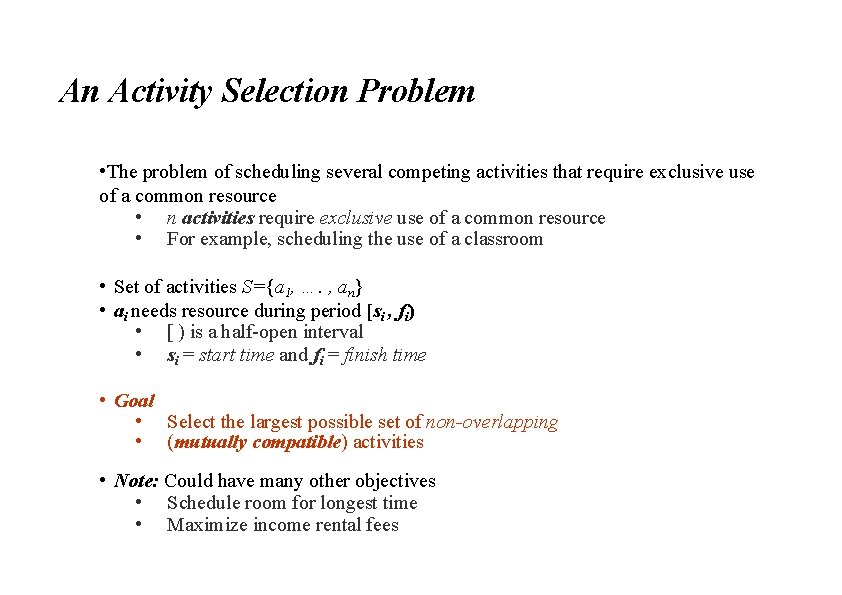
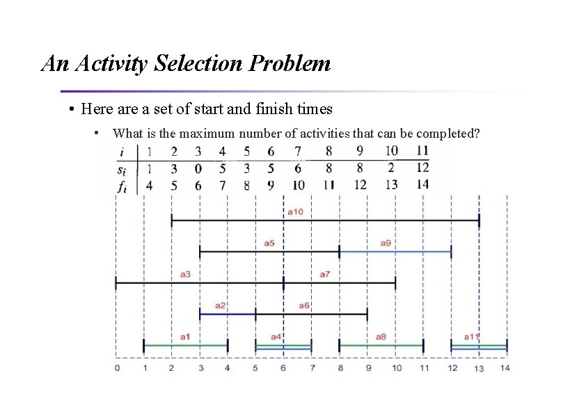
An Activity Selection Problem • The problem of scheduling several competing activities that require exclusive use of a common resource • n activities require exclusive use of a common resource • For example, scheduling the use of a classroom • Set of activities S={a 1, …. , an} • ai needs resource during period [si , fi) • [ ) is a half-open interval • si = start time and fi = finish time • Goal • Select the largest possible set of non-overlapping • (mutually compatible) activities • Note: Could have many other objectives • Schedule room for longest time • Maximize income rental fees

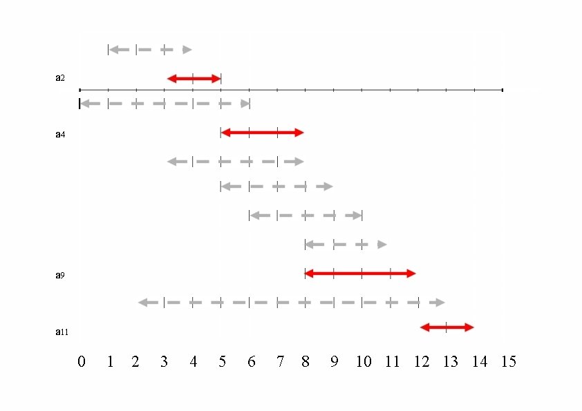
An Activity Selection Problem • Here a set of start and finish times • What is the maximum number of activities that can be completed?

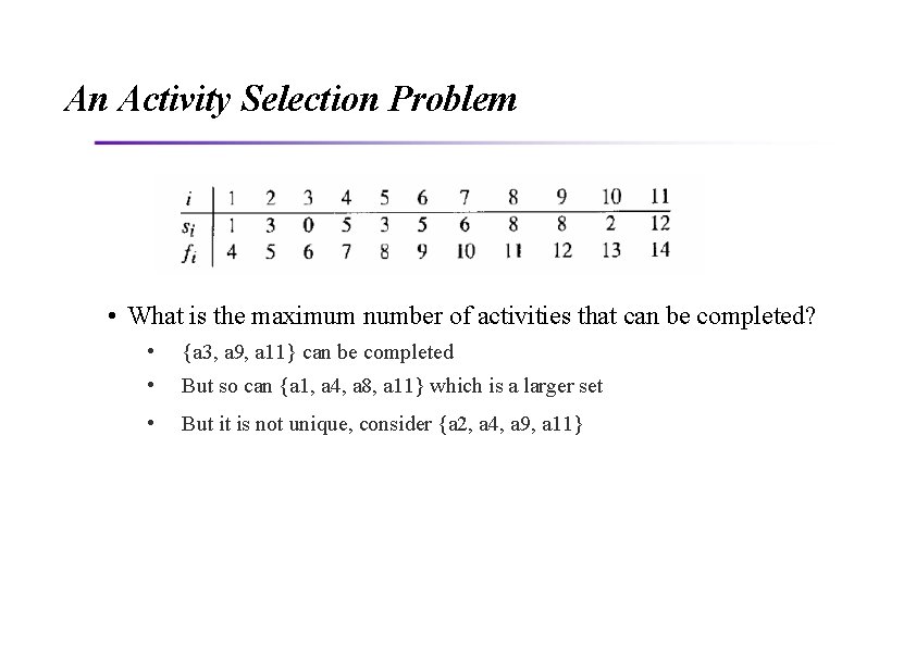
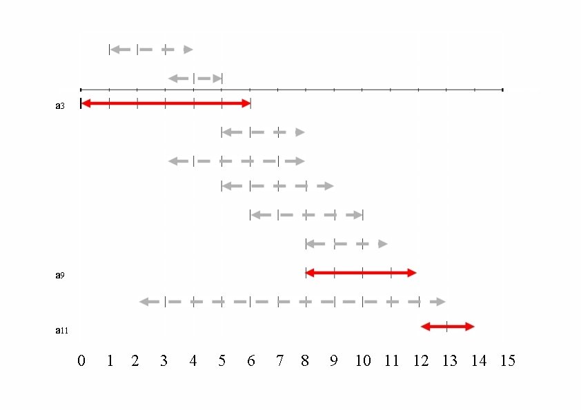
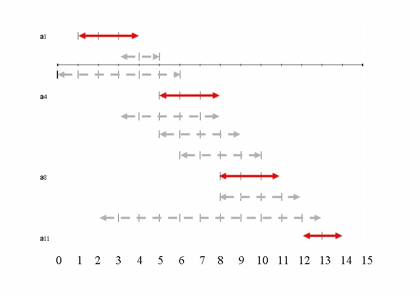
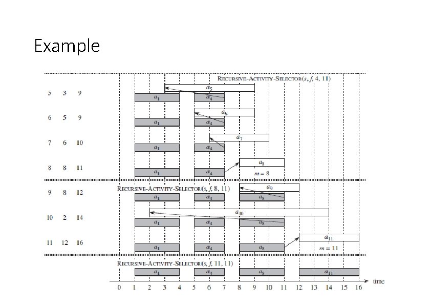
An Activity Selection Problem • What is the maximum number of activities that can be completed? • {a 3, a 9, a 11} can be completed • But so can {a 1, a 4, a 8, a 11} which is a larger set • But it is not unique, consider {a 2, a 4, a 9, a 11}

a 3 a 9 a 11 0 1 2 3 4 5 6 7 8 9 10 11 12 13 14 15

a 1 a 4 a 8 a 11 0 1 2 3 4 5 6 7 8 9 10 11 12 13 14 15

a 2 a 4 a 9 a 11 0 1 2 3 4 5 6 7 8 9 10 11 12 13 14 15

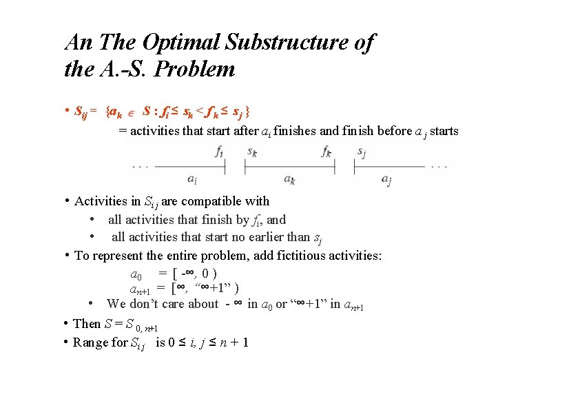
An The Optimal Substructure of the A. -S. Problem • Sij = {ak S : fi ≤ s k < f k ≤ s j } = activities that start after ai finishes and finish before a j starts • Activities in Si j are compatible with • all activities that finish by fi, and • all activities that start no earlier than sj • To represent the entire problem, add fictitious activities: a 0 = [ -∞, 0 ) an+1 = [∞, “∞+1” ) • We don’t care about - ∞ in a 0 or “∞+1” in an+1 • Then S = S 0, n+1 • Range for Si j is 0 ≤ i, j ≤ n + 1

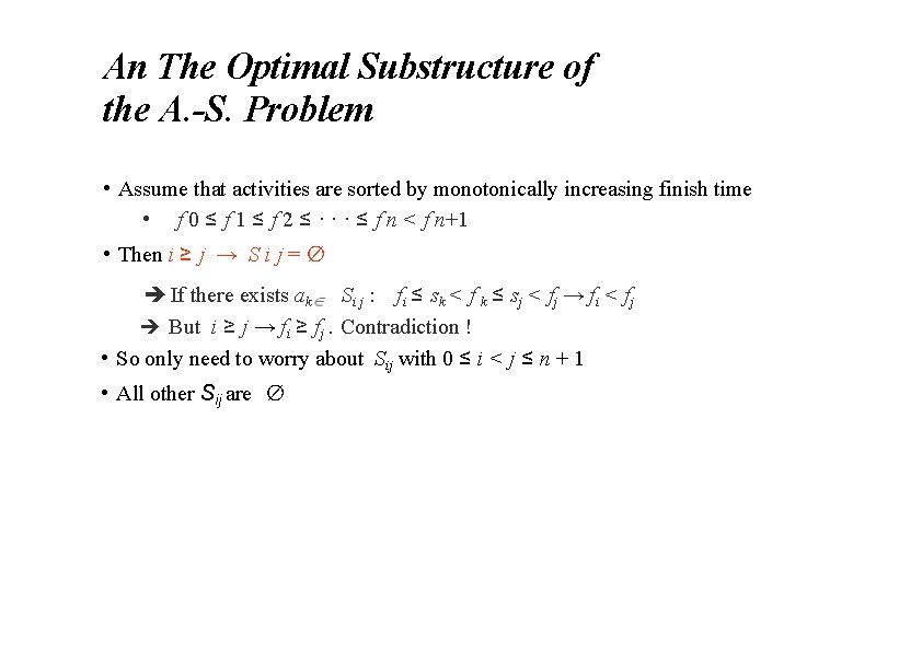
An The Optimal Substructure of the A. -S. Problem • Assume that activities are sorted by monotonically increasing finish time • f 0 ≤ f 1 ≤ f 2 ≤ · · · ≤ f n < f n+1 • Then i ≥ j → S i j = ∅ If there exists ak Si j : fi ≤ sk < f k ≤ sj < fj → fi < fj But i ≥ j → fi ≥ fj. Contradiction ! • So only need to worry about Sij with 0 ≤ i < j ≤ n + 1 • All other Sij are ∅

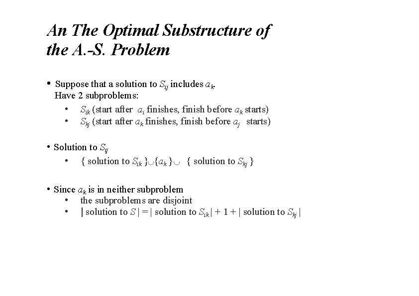
An The Optimal Substructure of the A. -S. Problem • Suppose that a solution to Sij includes ak. Have 2 subproblems: • Sik (start after ai finishes, finish before ak starts) • Skj (start after ak finishes, finish before aj starts) • Solution to Sij • { solution to Sik } {ak } { solution to Skj } • Since ak is in neither subproblem • the subproblems are disjoint • | solution to S | = | solution to Sik | + 1 + | solution to Skj |

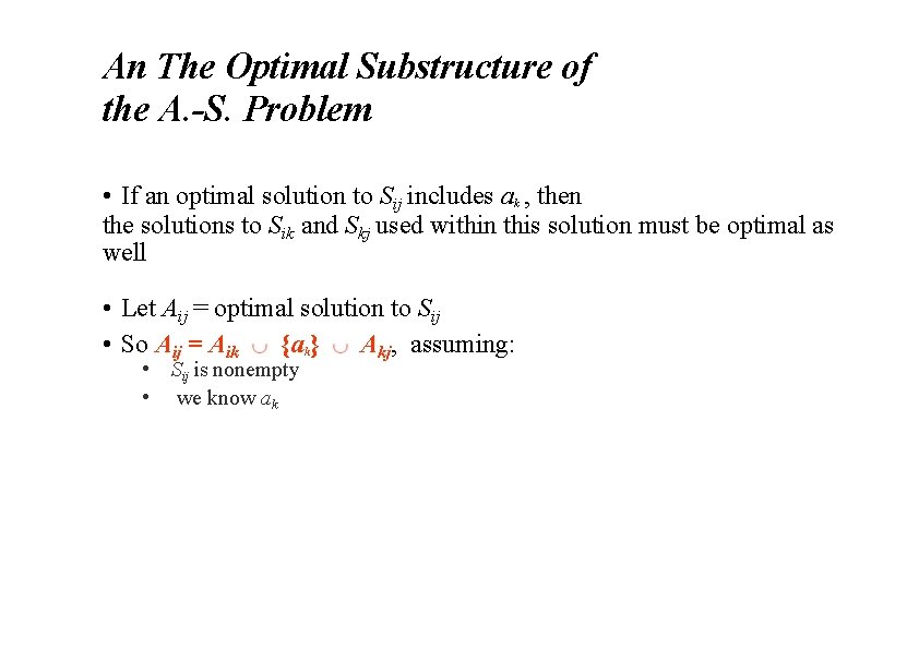
An The Optimal Substructure of the A. -S. Problem • If an optimal solution to Sij includes ak , then the solutions to Sik and Skj used within this solution must be optimal as well • Let Aij = optimal solution to Sij • So Aij = Aik {ak} Akj, assuming: • Sij is nonempty • we know ak
![An The Optimal Substructure of the A S Problem ci j size An The Optimal Substructure of the A. -S. Problem • c[i, j] : size](https://slidetodoc.com/presentation_image_h2/72f6856312335a18a79336dc6fd98326/image-14.jpg)
An The Optimal Substructure of the A. -S. Problem • c[i, j] : size of maximum-size subset of mutually compatible activities in Sij • i ≥ j → S i j = ∅→ c[i, j] = 0 • If Sij ≠ ∅, suppose we know that ak is in the subset • c [i, j] = c [i, k] + 1 + c [k, j]. • But, we don’t know which k to use, and so

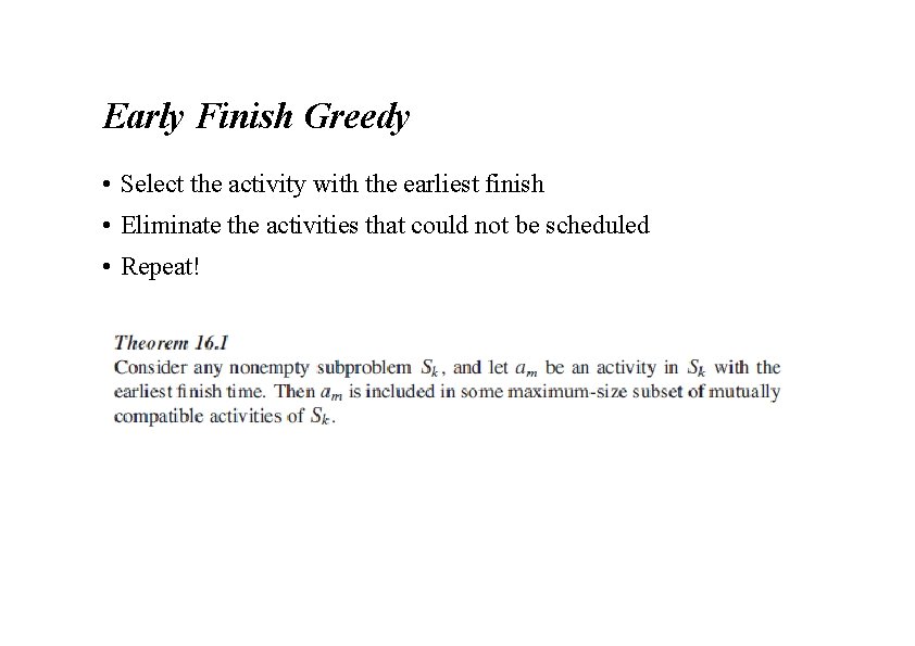
Early Finish Greedy • Select the activity with the earliest finish • Eliminate the activities that could not be scheduled • Repeat!

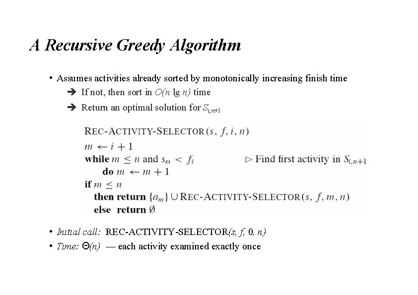
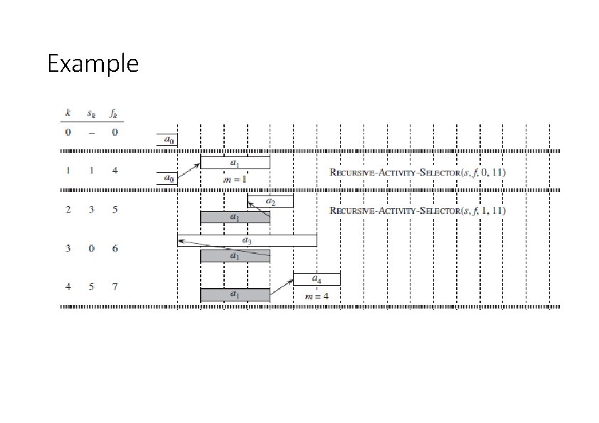
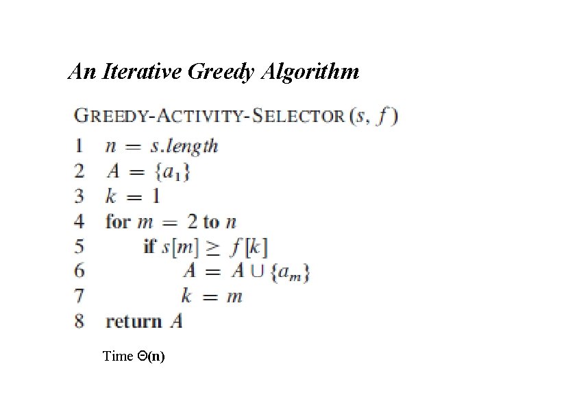
A Recursive Greedy Algorithm • Assumes activities already sorted by monotonically increasing finish time If not, then sort in O(n lg n) time Return an optimal solution for Si, n+1 • Initial call: REC-ACTIVITY-SELECTOR(s, f, 0, n) • Time: Θ(n) — each activity examined exactly once

Example

Example

An Iterative Greedy Algorithm Time Θ(n)

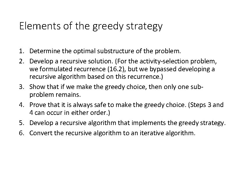
Elements of the greedy strategy 1. Determine the optimal substructure of the problem. 2. Develop a recursive solution. (For the activity-selection problem, we formulated recurrence (16. 2), but we bypassed developing a recursive algorithm based on this recurrence. ) 3. Show that if we make the greedy choice, then only one subproblem remains. 4. Prove that it is always safe to make the greedy choice. (Steps 3 and 4 can occur in either order. ) 5. Develop a recursive algorithm that implements the greedy strategy. 6. Convert the recursive algorithm to an iterative algorithm.

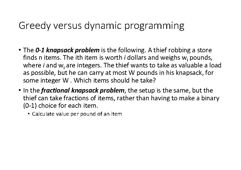
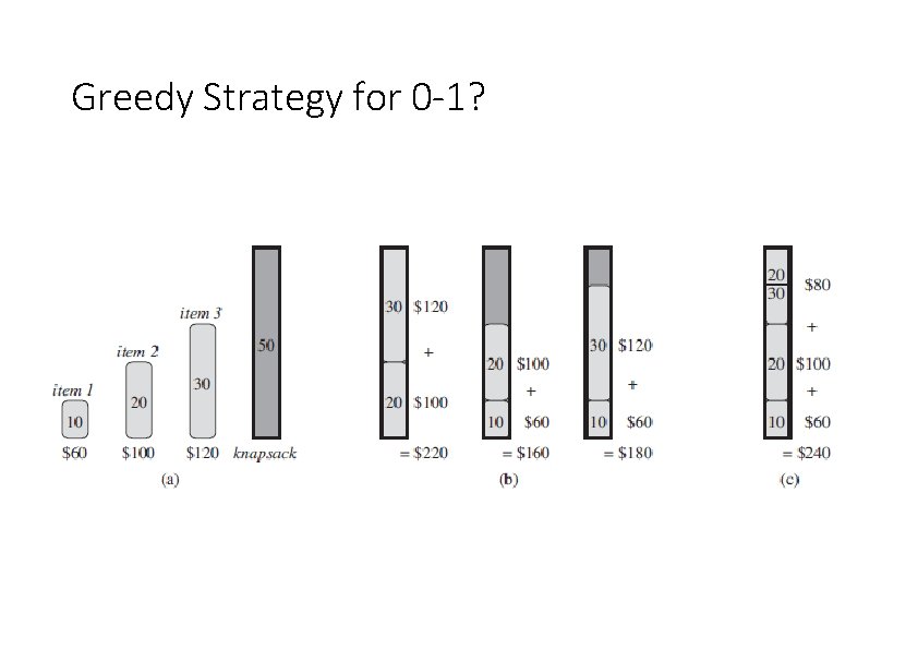
Greedy versus dynamic programming • The 0 -1 knapsack problem is the following. A thief robbing a store finds n items. The ith item is worth i dollars and weighs wi pounds, where i and wi are integers. The thief wants to take as valuable a load as possible, but he can carry at most W pounds in his knapsack, for some integer W. Which items should he take? • In the fractional knapsack problem, the setup is the same, but the thief can take fractions of items, rather than having to make a binary (0 -1) choice for each item. • Calculate value per pound of an item

Greedy Strategy for 0 -1?

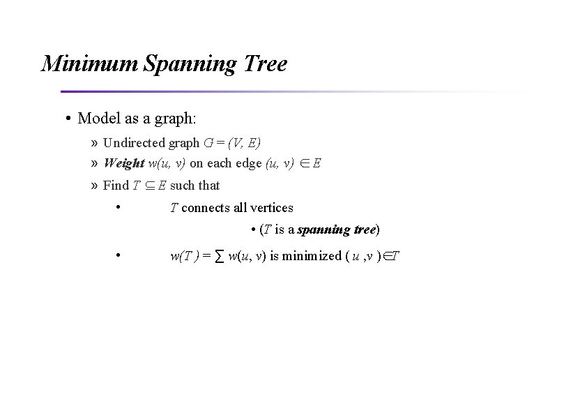
Minimum Spanning Tree • Model as a graph: » Undirected graph G = (V, E) » Weight w(u, v) on each edge (u, v) ∈ E » Find T ⊆ E such that • T connects all vertices • (T is a spanning tree) • w(T ) = ∑ w(u, v) is minimized ( u , v )∈T

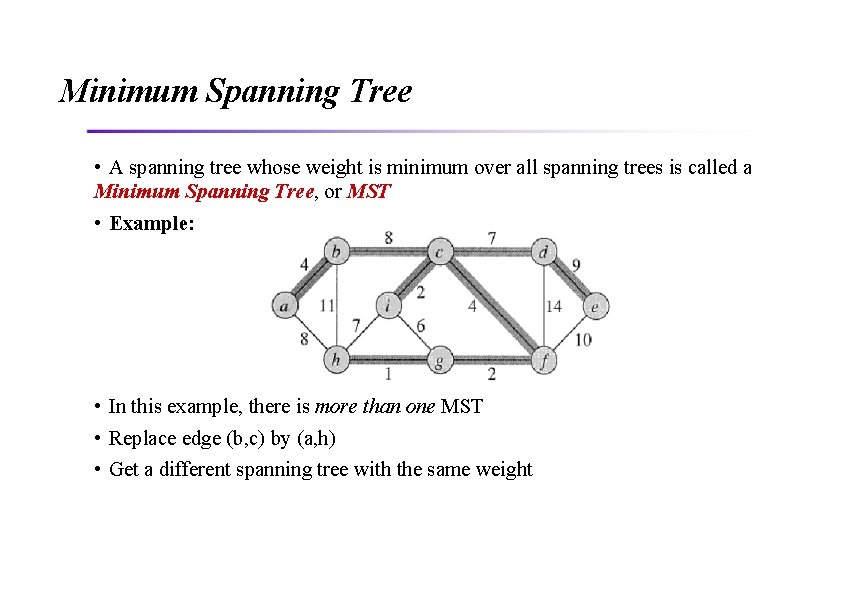
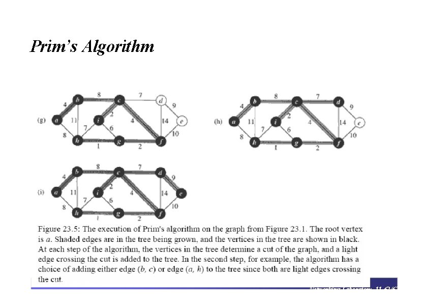
Minimum Spanning Tree • A spanning tree whose weight is minimum over all spanning trees is called a Minimum Spanning Tree, or MST • Example: • In this example, there is more than one MST • Replace edge (b, c) by (a, h) • Get a different spanning tree with the same weight

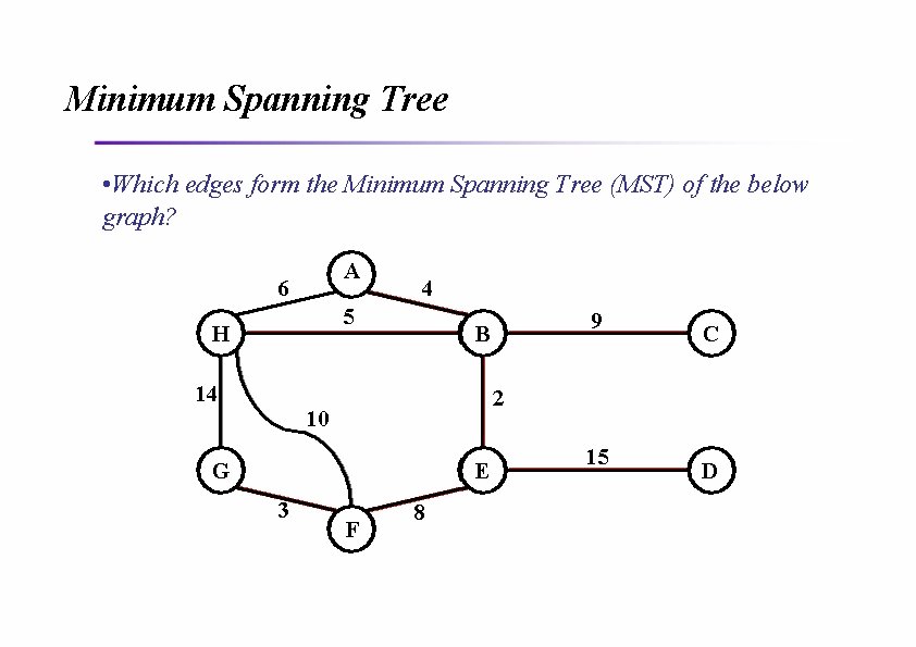
Minimum Spanning Tree • Which edges form the Minimum Spanning Tree (MST) of the below graph? A 6 4 5 H 14 C 2 10 G E 3 9 B F 8 15 D

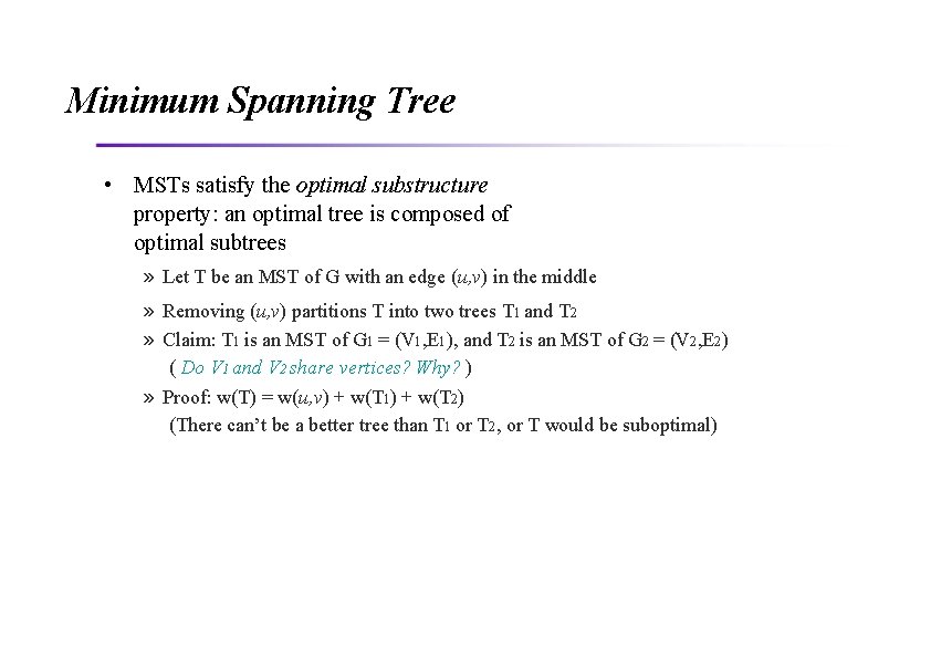
Minimum Spanning Tree • MSTs satisfy the optimal substructure property: an optimal tree is composed of optimal subtrees » Let T be an MST of G with an edge (u, v) in the middle » Removing (u, v) partitions T into two trees T 1 and T 2 » Claim: T 1 is an MST of G 1 = (V 1, E 1), and T 2 is an MST of G 2 = (V 2, E 2) ( Do V 1 and V 2 share vertices? Why? ) » Proof: w(T) = w(u, v) + w(T 1) + w(T 2) (There can’t be a better tree than T 1 or T 2, or T would be suboptimal)

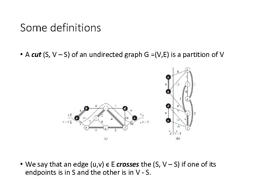
Some definitions • A cut (S, V – S) of an undirected graph G =(V, E) is a partition of V • We say that an edge (u, v) ϵ E crosses the (S, V – S) if one of its endpoints is in S and the other is in V - S.

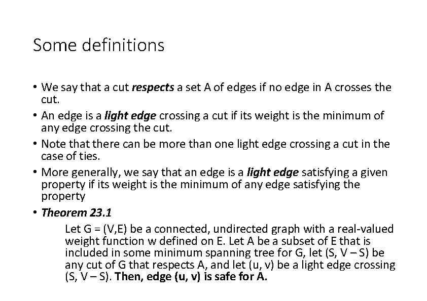
Some definitions • We say that a cut respects a set A of edges if no edge in A crosses the cut. • An edge is a light edge crossing a cut if its weight is the minimum of any edge crossing the cut. • Note that there can be more than one light edge crossing a cut in the case of ties. • More generally, we say that an edge is a light edge satisfying a given property if its weight is the minimum of any edge satisfying the property • Theorem 23. 1 Let G = (V, E) be a connected, undirected graph with a real-valued weight function w defined on E. Let A be a subset of E that is included in some minimum spanning tree for G, let (S, V – S) be any cut of G that respects A, and let (u, v) be a light edge crossing (S, V – S). Then, edge (u, v) is safe for A.

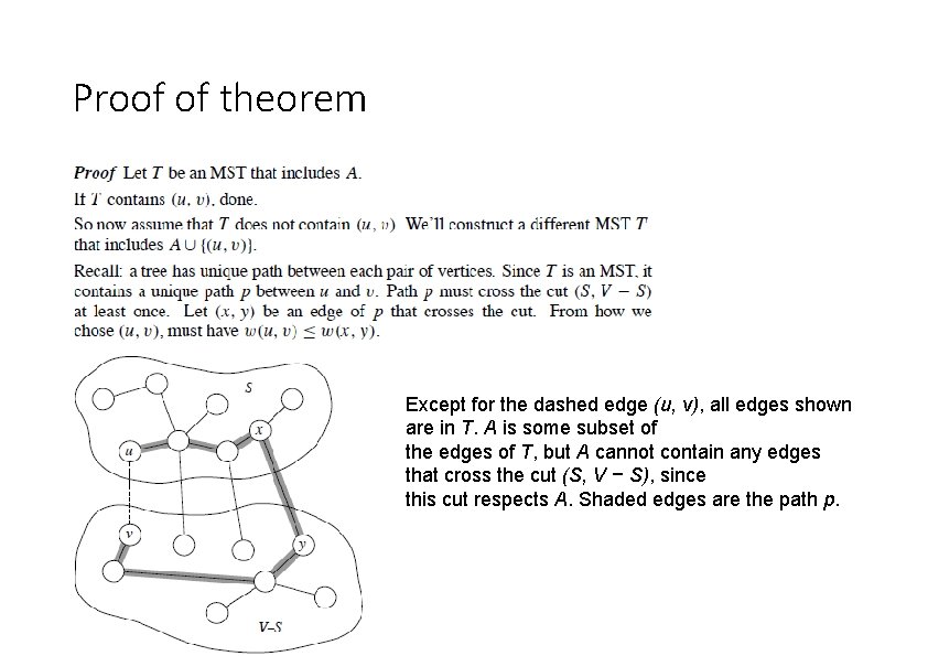
Proof of theorem Except for the dashed edge (u, v), all edges shown are in T. A is some subset of the edges of T, but A cannot contain any edges that cross the cut (S, V − S), since this cut respects A. Shaded edges are the path p.

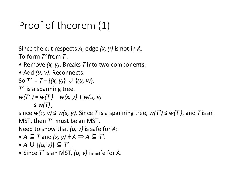
Proof of theorem (1) Since the cut respects A, edge (x, y) is not in A. To form T‘ from T : • Remove (x, y). Breaks T into two components. • Add (u, v). Reconnects. So T‘ = T − {(x, y)} ∪ {(u, v)}. T’ is a spanning tree. w(T’ ) = w(T ) − w(x, y) + w(u, v) ≤ w(T) , since w(u, v) ≤ w(x, y). Since T is a spanning tree, w(T’) ≤ w(T ), and T is an MST, then T’ must be an MST. Need to show that (u, v) is safe for A: • A ⊆ T and (x, y) ∉ A ⇒ A ⊆ T’. • A ∪ {(u, v)} ⊆ T’. • Since T’ is an MST, (u, v) is safe for A.

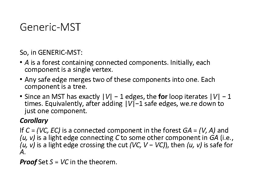
Generic-MST So, in GENERIC-MST: • A is a forest containing connected components. Initially, each component is a single vertex. • Any safe edge merges two of these components into one. Each component is a tree. • Since an MST has exactly |V| − 1 edges, the for loop iterates |V| − 1 times. Equivalently, after adding |V|− 1 safe edges, we. re down to just one component. Corollary If C = (VC, EC) is a connected component in the forest GA = (V, A) and (u, v) is a light edge connecting C to some other component in GA (i. e. , (u, v) is a light edge crossing the cut (VC, V − VC)), then (u, v) is safe for A. Proof Set S = VC in theorem.

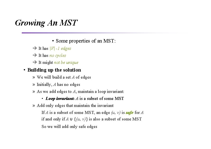
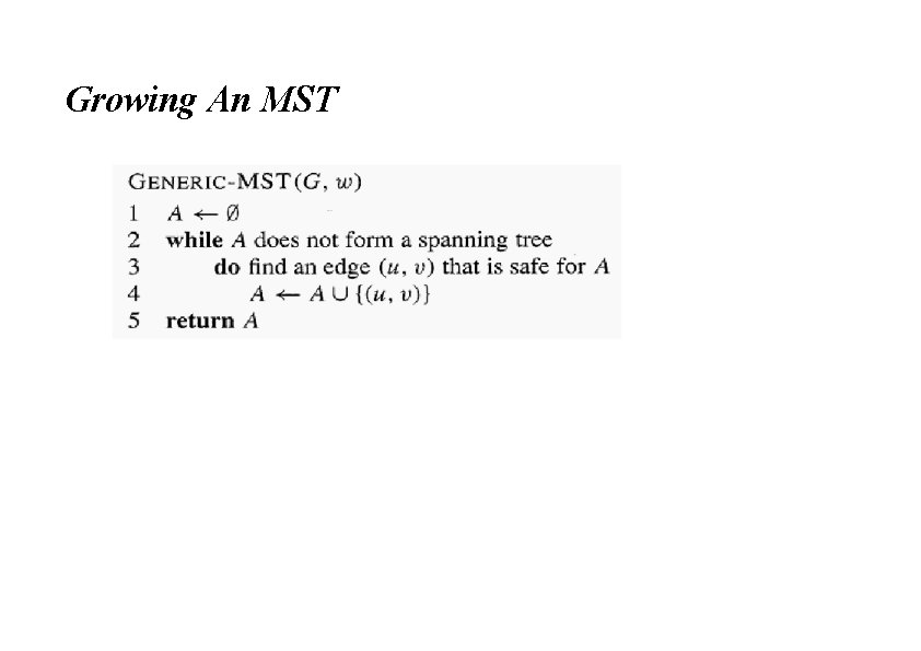
Growing An MST • Some properties of an MST: It has |V| -1 edges It has no cycles It might not be unique • Building up the solution » We will build a set A of edges » Initially, A has no edges » As we add edges to A, maintain a loop invariant: • Loop invariant: A is a subset of some MST » Add only edges that maintain the invariant If A is a subset of some MST, an edge (u, v) is safe for A if and only if A υ {(u, v)} is also a subset of some MST So we will add only safe edges

Growing An MST

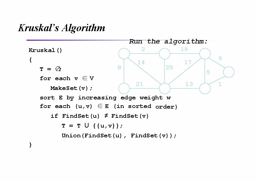
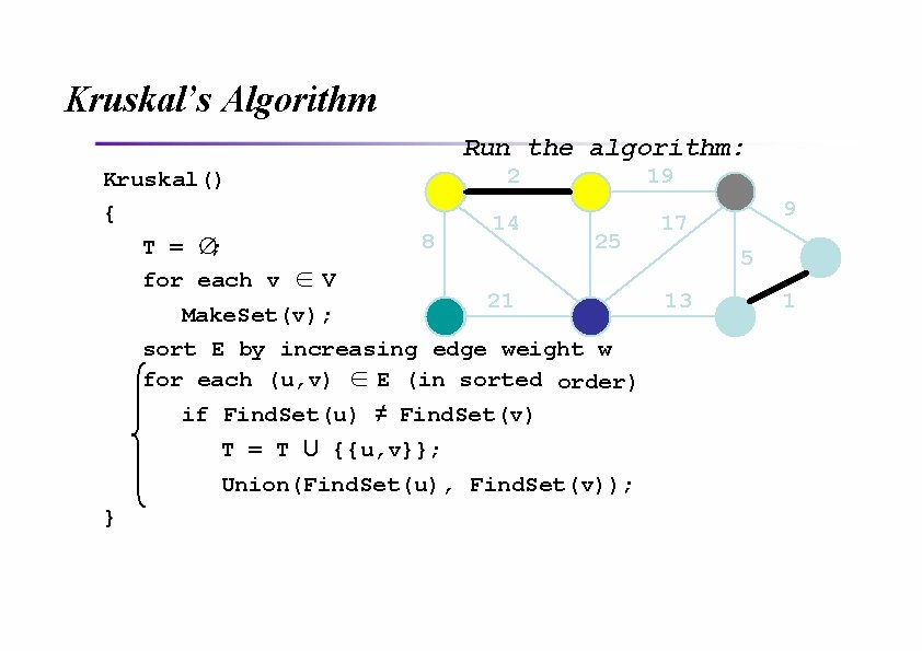
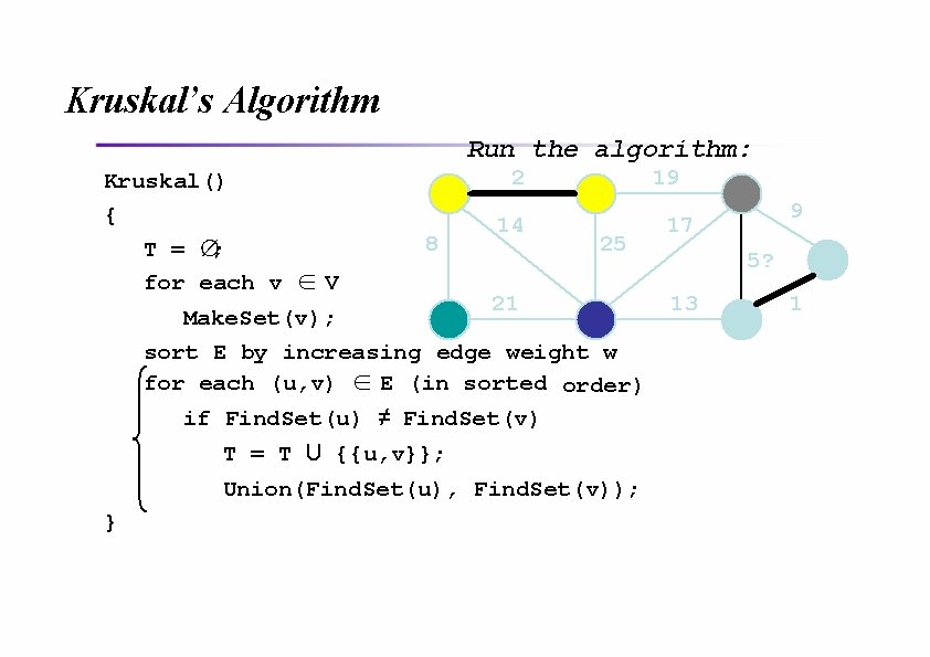
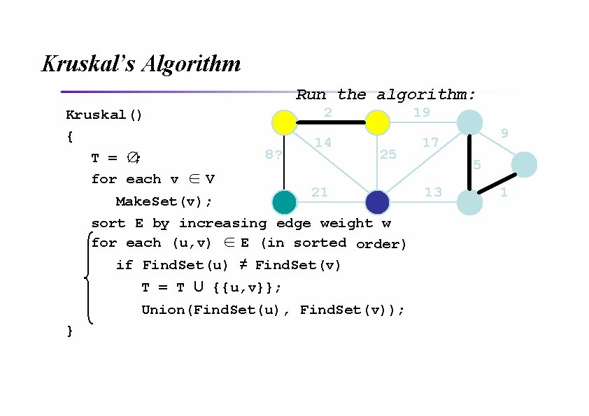
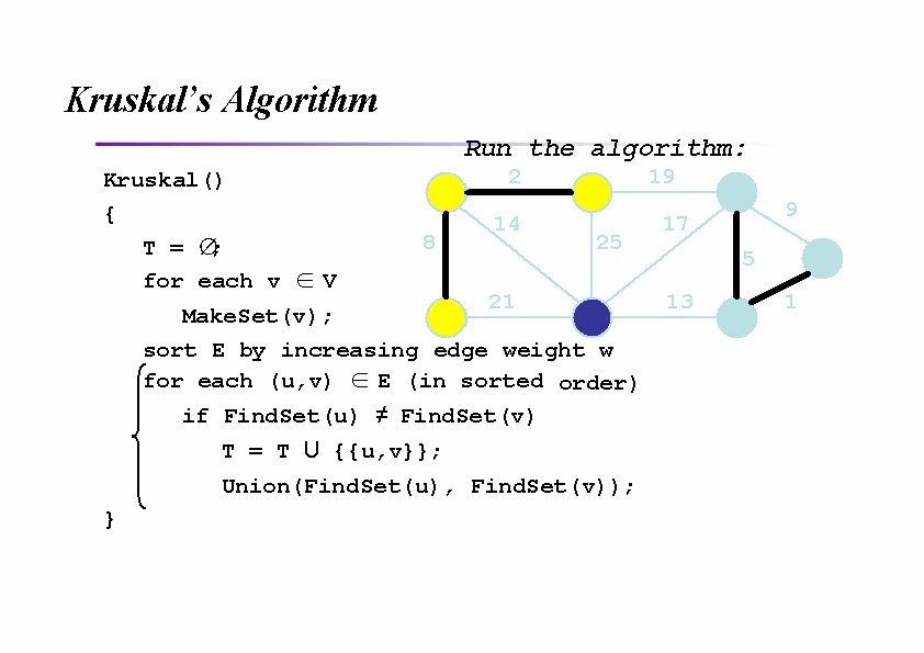
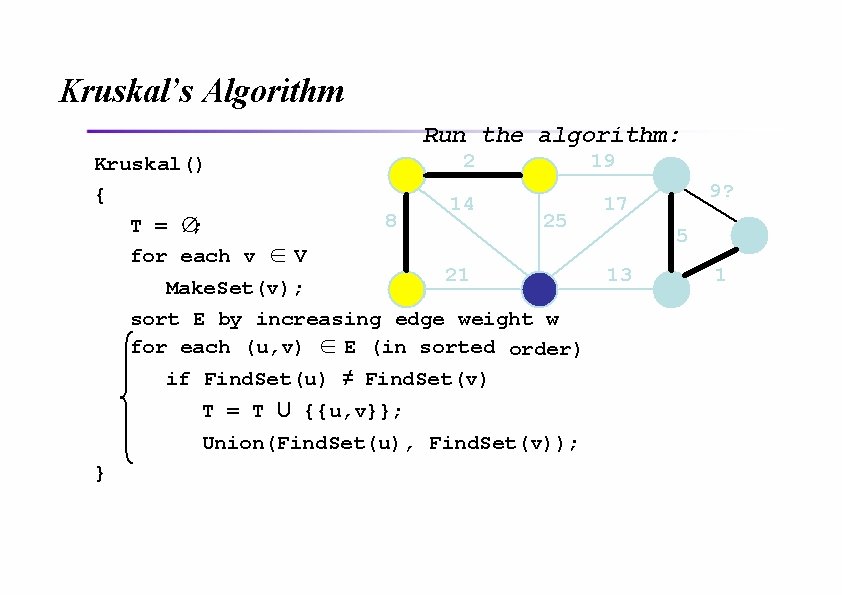
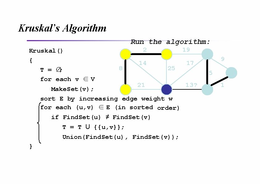
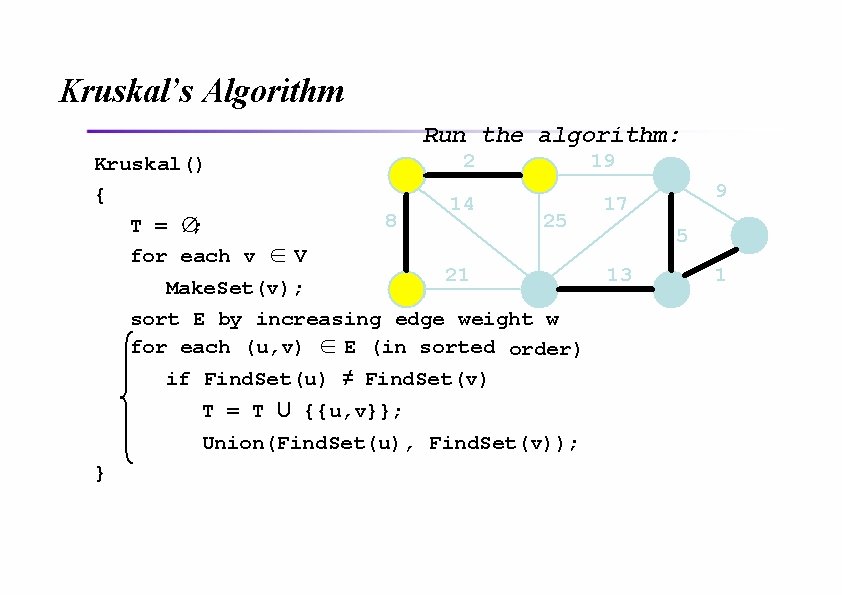
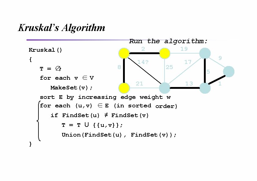
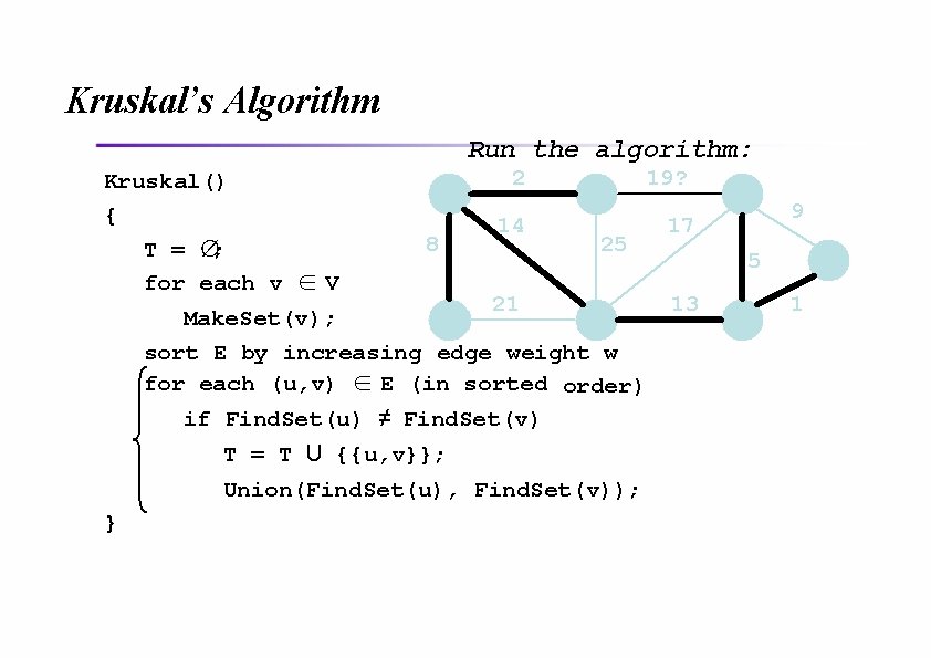
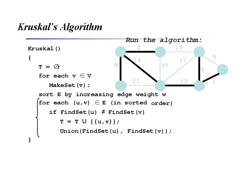
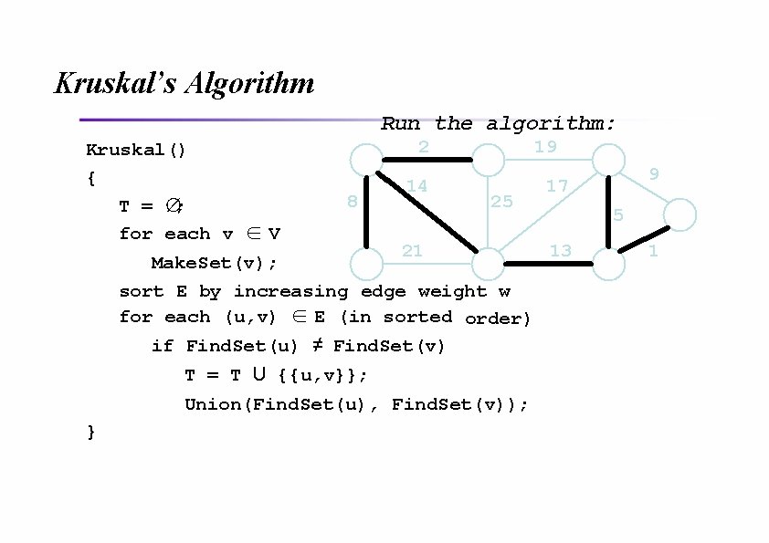
Kruskal’s Algorithm Run the algorithm: Kruskal() { T = ∅; for each v ∈ V 2 8 14 19 25 21 Make. Set(v); sort E by increasing edge weight w for each (u, v) ∈ E (in sorted order) if Find. Set(u) ≠ Find. Set(v) T = T U {{u, v}}; Union(Find. Set(u), Find. Set(v)); } 9 17 5 13 1

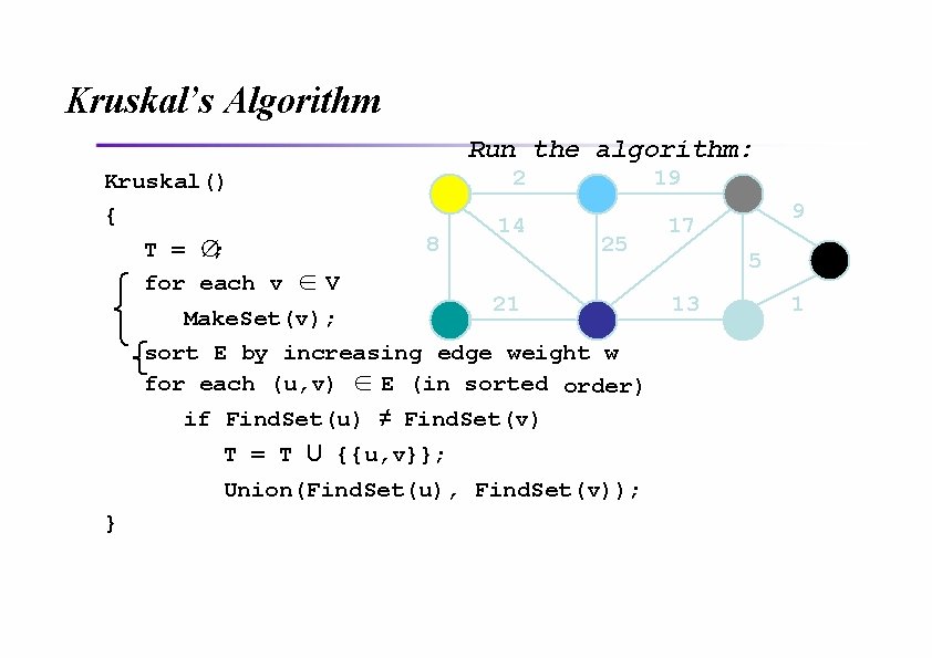
Kruskal’s Algorithm Run the algorithm: Kruskal() { T = ∅; for each v ∈ V 2 8 14 19 25 21 Make. Set(v); sort E by increasing edge weight w for each (u, v) ∈ E (in sorted order) if Find. Set(u) ≠ Find. Set(v) T = T U {{u, v}}; Union(Find. Set(u), Find. Set(v)); } 9 17 5 13 1

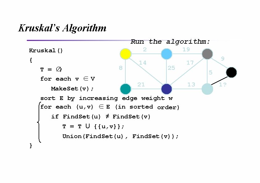
Kruskal’s Algorithm Run the algorithm: Kruskal() { T = ∅; for each v ∈ V 2 8 14 19 25 21 Make. Set(v); sort E by increasing edge weight w for each (u, v) ∈ E (in sorted order) if Find. Set(u) ≠ Find. Set(v) T = T U {{u, v}}; Union(Find. Set(u), Find. Set(v)); } 9 17 5 13 1?

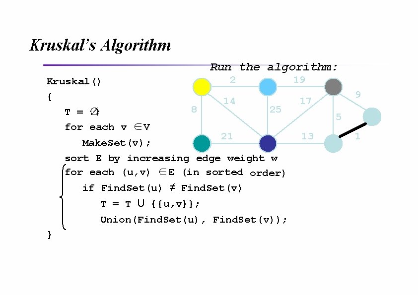
Kruskal’s Algorithm Run the algorithm: Kruskal() { T = ∅; for each v ∈V 2 8 14 19 25 21 Make. Set(v); sort E by increasing edge weight w for each (u, v) ∈E (in sorted order) if Find. Set(u) ≠ Find. Set(v) T = T U {{u, v}}; Union(Find. Set(u), Find. Set(v)); } 9 17 5 13 1

Kruskal’s Algorithm Run the algorithm: Kruskal() { T = ∅; for each v ∈ V 2? 8 14 19 25 21 Make. Set(v); sort E by increasing edge weight w for each (u, v) ∈ E (in sorted order) if Find. Set(u) ≠ Find. Set(v) T = T U {{u, v}}; Union(Find. Set(u), Find. Set(v)); } 9 17 5 13 1

Kruskal’s Algorithm Run the algorithm: Kruskal() { T = ∅; for each v ∈ V 2 8 14 19 25 21 Make. Set(v); sort E by increasing edge weight w for each (u, v) ∈ E (in sorted order) if Find. Set(u) ≠ Find. Set(v) T = T U {{u, v}}; Union(Find. Set(u), Find. Set(v)); } 9 17 5 13 1

Kruskal’s Algorithm Run the algorithm: Kruskal() { T = ∅; for each v ∈ V 2 8 14 19 25 21 Make. Set(v); sort E by increasing edge weight w for each (u, v) ∈ E (in sorted order) if Find. Set(u) ≠ Find. Set(v) T = T U {{u, v}}; Union(Find. Set(u), Find. Set(v)); } 9 17 5? 13 1

Kruskal’s Algorithm Run the algorithm: Kruskal() { T = ∅; for each v ∈ V 2 8 14 19 25 21 Make. Set(v); sort E by increasing edge weight w for each (u, v) ∈ E (in sorted order) if Find. Set(u) ≠ Find. Set(v) T = T U {{u, v}}; Union(Find. Set(u), Find. Set(v)); } 9 17 5 13 1

Kruskal’s Algorithm Run the algorithm: Kruskal() { T = ∅; for each v ∈ V 2 8? 14 19 25 21 Make. Set(v); sort E by increasing edge weight w for each (u, v) ∈ E (in sorted order) if Find. Set(u) ≠ Find. Set(v) T = T U {{u, v}}; Union(Find. Set(u), Find. Set(v)); } 9 17 5 13 1

Kruskal’s Algorithm Run the algorithm: Kruskal() { T = ∅; for each v ∈ V 2 8 14 19 25 21 Make. Set(v); sort E by increasing edge weight w for each (u, v) ∈ E (in sorted order) if Find. Set(u) ≠ Find. Set(v) T = T U {{u, v}}; Union(Find. Set(u), Find. Set(v)); } 9 17 5 13 1

Kruskal’s Algorithm Run the algorithm: Kruskal() { T = ∅; for each v ∈ V 2 8 14 19 25 21 Make. Set(v); sort E by increasing edge weight w for each (u, v) ∈ E (in sorted order) if Find. Set(u) ≠ Find. Set(v) T = T U {{u, v}}; Union(Find. Set(u), Find. Set(v)); } 9? 17 5 13 1

Kruskal’s Algorithm Run the algorithm: Kruskal() { T = ∅; for each v ∈ V 2 8 14 19 25 21 Make. Set(v); sort E by increasing edge weight w for each (u, v) ∈ E (in sorted order) if Find. Set(u) ≠ Find. Set(v) T = T U {{u, v}}; Union(Find. Set(u), Find. Set(v)); } 9 17 5 13 1

Kruskal’s Algorithm Run the algorithm: Kruskal() { T = ∅; for each v ∈ V 2 8 14 19 25 21 13? Make. Set(v); sort E by increasing edge weight w for each (u, v) ∈ E (in sorted order) if Find. Set(u) ≠ Find. Set(v) T = T U {{u, v}}; Union(Find. Set(u), Find. Set(v)); } 9 17 5 1

Kruskal’s Algorithm Run the algorithm: Kruskal() { T = ∅; for each v ∈ V 2 8 14 19 25 21 Make. Set(v); sort E by increasing edge weight w for each (u, v) ∈ E (in sorted order) if Find. Set(u) ≠ Find. Set(v) T = T U {{u, v}}; Union(Find. Set(u), Find. Set(v)); } 9 17 5 13 1

Kruskal’s Algorithm Run the algorithm: Kruskal() { T = ∅; for each v ∈ V 2 8 14? 19 25 21 Make. Set(v); sort E by increasing edge weight w for each (u, v) ∈ E (in sorted order) if Find. Set(u) ≠ Find. Set(v) T = T U {{u, v}}; Union(Find. Set(u), Find. Set(v)); } 9 17 5 13 1

Kruskal’s Algorithm Run the algorithm: Kruskal() { T = ∅; for each v ∈ V 2 8 14 19 25 21 Make. Set(v); sort E by increasing edge weight w for each (u, v) ∈ E (in sorted order) if Find. Set(u) ≠ Find. Set(v) T = T U {{u, v}}; Union(Find. Set(u), Find. Set(v)); } 9 17 5 13 1

Kruskal’s Algorithm Run the algorithm: Kruskal() { T = ∅; for each v ∈ V 2 8 14 19 25 21 Make. Set(v); sort E by increasing edge weight w for each (u, v) ∈ E (in sorted order) if Find. Set(u) ≠ Find. Set(v) T = T U {{u, v}}; Union(Find. Set(u), Find. Set(v)); } 9 17? 5 13 1

Kruskal’s Algorithm Run the algorithm: Kruskal() { T = ∅; for each v ∈ V 2 8 14 19? 25 21 Make. Set(v); sort E by increasing edge weight w for each (u, v) ∈ E (in sorted order) if Find. Set(u) ≠ Find. Set(v) T = T U {{u, v}}; Union(Find. Set(u), Find. Set(v)); } 9 17 5 13 1

Kruskal’s Algorithm Run the algorithm: Kruskal() { T = ∅; for each v ∈ V 2 8 14 19 25 21? Make. Set(v); sort E by increasing edge weight w for each (u, v) ∈ E (in sorted order) if Find. Set(u) ≠ Find. Set(v) T = T U {{u, v}}; Union(Find. Set(u), Find. Set(v)); } 9 17 5 13 1

Kruskal’s Algorithm Run the algorithm: Kruskal() { T = ∅; for each v ∈ V 2 8 14 19 25? 21 Make. Set(v); sort E by increasing edge weight w for each (u, v) ∈ E (in sorted order) if Find. Set(u) ≠ Find. Set(v) T = T U {{u, v}}; Union(Find. Set(u), Find. Set(v)); } 9 17 5 13 1

Kruskal’s Algorithm Run the algorithm: Kruskal() { T = ∅; for each v ∈ V 2 8 14 19 25 21 Make. Set(v); sort E by increasing edge weight w for each (u, v) ∈ E (in sorted order) if Find. Set(u) ≠ Find. Set(v) T = T U {{u, v}}; Union(Find. Set(u), Find. Set(v)); } 9 17 5 13 1

Kruskal’s Algorithm Run the algorithm: Kruskal() { T = ∅; for each v ∈ V 2 8 14 19 25 21 13 Make. Set(v); sort E by increasing edge weight w for each (u, v) ∈ E (in sorted order) if Find. Set(u) ≠ Find. Set(v) T = T U {{u, v}}; Union(Find. Set(u), Find. Set(v)); } 9 17 5 1

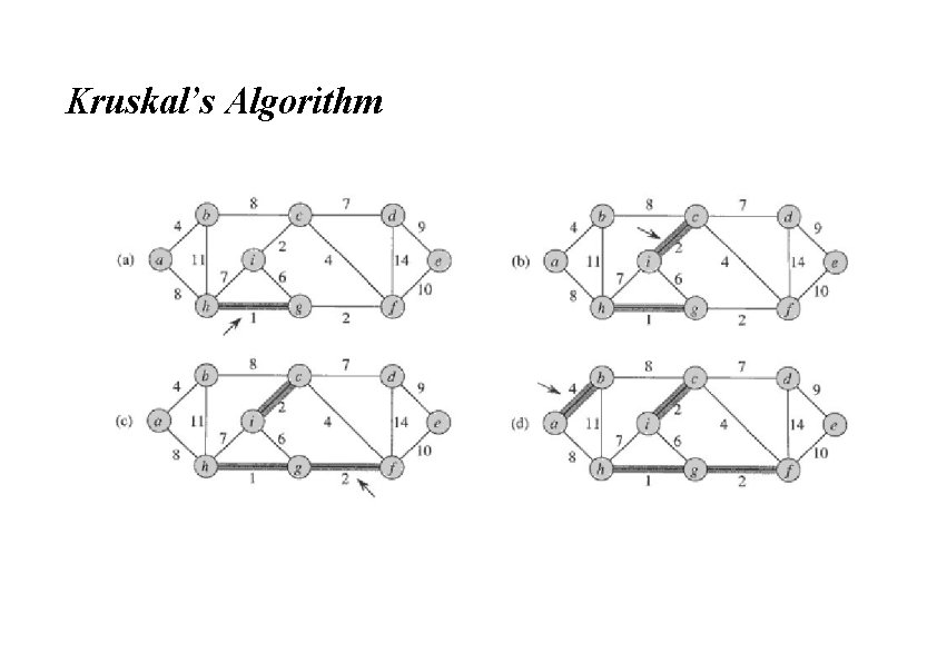
Kruskal’s Algorithm

Kruskal’s Algorithm

Kruskal’s Algorithm Spring 2006 Algorithm Networking Laboratory 11 -37/62

Kruskal’s Algorithm What will affect the running time? Kruskal() 1 Sort { O(V) Make. Set() calls T = ∅; O(E) Find. Set() calls for each v ∈ V O(V) Union() calls Make. Set(v); (Exactly how many Union()s? ) sort E by increasing edge weight w for each (u, v) ∈ E (in sorted order) if Find. Set(u) ≠ Find. Set(v) T = T U {{u, v}}; Union(Find. Set(u), Find. Set(v)); }
![Prims Algorithm MSTPrimG w r 6 Q VG 4 for each u Prim’s Algorithm MST-Prim(G, w, r) 6 Q = V[G]; 4 for each u ∈](https://slidetodoc.com/presentation_image_h2/72f6856312335a18a79336dc6fd98326/image-60.jpg)
Prim’s Algorithm MST-Prim(G, w, r) 6 Q = V[G]; 4 for each u ∈ Q key[u] = ∞; key[r] = 0; 9 5 14 2 10 15 П[r] = NULL; while (Q not empty) u = Extract. Min(Q); for each v ∈ Adj[u] 3 8 Run on example graph if (v ∈ Q and w(u, v) < key[v]) П[v] = u; key[v] = w(u, v);
![Prims Algorithm r Q VG 14 Пr NULL while Prim’s Algorithm • r) Q = V[G]; 14 • П[r] = NULL; • while](https://slidetodoc.com/presentation_image_h2/72f6856312335a18a79336dc6fd98326/image-61.jpg)
Prim’s Algorithm • r) Q = V[G]; 14 • П[r] = NULL; • while (Q not empty) • u = Extract. Min(Q); for each v ∈ Adj[u] • if (v ∈ Q and w(u, v) < • П[v] = u; • key[v] = w(u, v); 4 5 ∞ • for each u ∈ Q • key[u] = ∞; • key[r] = 0; ∞ 6 MST-Prim(G, w, ∞ ∞ 2 10 ∞ ∞ 3 9 ∞ 15 8 Run on example graph key[v]) ∞
![Prims Algorithm r Q VG 14 r Пr NULL Prim’s Algorithm • r) Q = V[G]; 14 r • П[r] = NULL; •](https://slidetodoc.com/presentation_image_h2/72f6856312335a18a79336dc6fd98326/image-62.jpg)
Prim’s Algorithm • r) Q = V[G]; 14 r • П[r] = NULL; • while (Q not empty) • u = Extract. Min(Q); for each v ∈Adj[u] • if (v ∈Q and w(u, v) < • П[v] = u; • key[v] = w(u, v); 4 5 ∞ • for each u ∈ Q • key[u] = ∞; • key[r] = 0; ∞ 6 MST-Prim(G, w, ∞ ∞ 2 10 0 ∞ 3 9 ∞ 15 8 Pick a start vertex r key[v]) ∞
![Prims Algorithm MSTPrimG w r Q VG keyu keyr 0 Prim’s Algorithm MST-Prim(G, w, r) Q = V[G]; key[u] = ∞; key[r] = 0;](https://slidetodoc.com/presentation_image_h2/72f6856312335a18a79336dc6fd98326/image-63.jpg)
Prim’s Algorithm MST-Prim(G, w, r) Q = V[G]; key[u] = ∞; key[r] = 0; 14 u while (Q not empty) u = Extract. Min(Q); for each v ∈Adj[u] ∞ 0 ∞ 3 9 ∞ 2 10 ∞ 15 ∞ 8 Black vertices have been removed from Q if (v ∈Q and w(u, v) < key[v]) П[v] = u; key[v] = w(u, v); 4 5 ∞ for each u ∈Q П[r] = NULL; ∞ 6
![Prims Algorithm r Q VG 14 u Пr NULL Prim’s Algorithm • r) Q = V[G]; 14 u • П[r] = NULL; •](https://slidetodoc.com/presentation_image_h2/72f6856312335a18a79336dc6fd98326/image-64.jpg)
Prim’s Algorithm • r) Q = V[G]; 14 u • П[r] = NULL; • while (Q not empty) • u = Extract. Min(Q); for each v ∈Adj[u] • if (v ∈Q and w(u, v) < • П[v] = u; • key[v] = w(u, v); 4 5 ∞ • for each u ∈ Q • key[u] = ∞; • key[r] = 0; ∞ 6 MST-Prim(G, w, ∞ ∞ 2 10 0 ∞ 3 9 3 15 ∞ 8 Black arrows indicate parent pointers key[v])
![Prims Algorithm MSTPrimG w r 6 Q VG keyu keyr Prim’s Algorithm MST-Prim(G, w, r) ∞ 6 Q = V[G]; key[u] = ∞; key[r]](https://slidetodoc.com/presentation_image_h2/72f6856312335a18a79336dc6fd98326/image-65.jpg)
Prim’s Algorithm MST-Prim(G, w, r) ∞ 6 Q = V[G]; key[u] = ∞; key[r] = 0; 14 u П[r] = NULL; 5 14 for each u ∈Q while (Q not empty) u = Extract. Min(Q); key[v] = w(u, v); ∞ 0 ∞ 3 9 ∞ 2 10 3 for each v ∈Adj[u] if (v ∈Q and w(u, v) < key[v]) П[v] = u; 4 8 15 ∞
![Prims Algorithm MSTPrimG w r 6 Q VG for each u Q Prim’s Algorithm MST-Prim(G, w, r) ∞ 6 Q = V[G]; for each u ∈Q](https://slidetodoc.com/presentation_image_h2/72f6856312335a18a79336dc6fd98326/image-66.jpg)
Prim’s Algorithm MST-Prim(G, w, r) ∞ 6 Q = V[G]; for each u ∈Q key[u] = ∞; key[r] = 0; 4 5 14 14 ∞ while (Q not empty) u = Extract. Min(Q); for each v ∈Adj[u] ∞ 3 u 3 if (v ∈Q and w(u, v) < key[v]) П[v] = u; key[v] = w(u, v); ∞ 2 10 0 П[r] = NULL; 9 8 15 ∞
![Prims Algorithm MSTPrimG w r 6 Q VG for each u Q Prim’s Algorithm MST-Prim(G, w, r) ∞ 6 Q = V[G]; for each u ∈Q](https://slidetodoc.com/presentation_image_h2/72f6856312335a18a79336dc6fd98326/image-67.jpg)
Prim’s Algorithm MST-Prim(G, w, r) ∞ 6 Q = V[G]; for each u ∈Q key[u] = ∞; key[r] = 0; 4 5 14 14 ∞ while (Q not empty) u = Extract. Min(Q); for each v ∈Adj[u] 8 3 u 3 if (v ∈Q and w(u, v) < key[v]) П[v] = u; key[v] = w(u, v); ∞ 2 10 0 П[r] = NULL; 9 8 15 ∞
![Prims Algorithm MSTPrimG w r 6 Q VG for each u Q Prim’s Algorithm MST-Prim(G, w, r) ∞ 6 Q = V[G]; for each u ∈Q](https://slidetodoc.com/presentation_image_h2/72f6856312335a18a79336dc6fd98326/image-68.jpg)
Prim’s Algorithm MST-Prim(G, w, r) ∞ 6 Q = V[G]; for each u ∈Q key[u] = ∞; key[r] = 0; 4 5 10 14 ∞ while (Q not empty) u = Extract. Min(Q); for each v ∈Adj[u] 8 3 u 3 if (v ∈Q and w(u, v) < key[v]) П[v] = u; key[v] = w(u, v); ∞ 2 10 0 П[r] = NULL; 9 8 15 ∞
![Prims Algorithm MSTPrimG w r 6 Q VG for each u Q Prim’s Algorithm MST-Prim(G, w, r) ∞ 6 Q = V[G]; for each u ∈Q](https://slidetodoc.com/presentation_image_h2/72f6856312335a18a79336dc6fd98326/image-69.jpg)
Prim’s Algorithm MST-Prim(G, w, r) ∞ 6 Q = V[G]; for each u ∈Q key[u] = ∞; key[r] = 0; 4 5 10 14 ∞ while (Q not empty) u = Extract. Min(Q); 8 3 3 for each v ∈Adj[u] if (v ∈Q and w(u, v) < key[v]) П[v] = u; key[v] = w(u, v); ∞ 2 10 0 П[r] = NULL; 9 8 u 15 ∞
![Prims Algorithm MSTPrimG w r 6 Q VG for each u Q Prim’s Algorithm MST-Prim(G, w, r) ∞ 6 Q = V[G]; for each u ∈Q](https://slidetodoc.com/presentation_image_h2/72f6856312335a18a79336dc6fd98326/image-70.jpg)
Prim’s Algorithm MST-Prim(G, w, r) ∞ 6 Q = V[G]; for each u ∈Q key[u] = ∞; key[r] = 0; 4 5 10 14 2 while (Q not empty) u = Extract. Min(Q); 8 3 3 for each v ∈Adj[u] if (v ∈Q and w(u, v) < key[v]) П[v] = u; key[v] = w(u, v); ∞ 2 10 0 П[r] = NULL; 9 8 u 15 ∞
![Prims Algorithm MSTPrimG w r 6 Q VG for each u Q Prim’s Algorithm MST-Prim(G, w, r) ∞ 6 Q = V[G]; for each u ∈Q](https://slidetodoc.com/presentation_image_h2/72f6856312335a18a79336dc6fd98326/image-71.jpg)
Prim’s Algorithm MST-Prim(G, w, r) ∞ 6 Q = V[G]; for each u ∈Q key[u] = ∞; key[r] = 0; 4 5 10 14 2 while (Q not empty) u = Extract. Min(Q); 8 3 3 for each v ∈Adj[u] if (v ∈Q and w(u, v) < key[v]) П[v] = u; key[v] = w(u, v); ∞ 2 10 0 П[r] = NULL; 9 8 u 15 15
![Prims Algorithm MSTPrimG w r 6 Q VG for each u Q Prim’s Algorithm MST-Prim(G, w, r) ∞ 6 Q = V[G]; for each u ∈Q](https://slidetodoc.com/presentation_image_h2/72f6856312335a18a79336dc6fd98326/image-72.jpg)
Prim’s Algorithm MST-Prim(G, w, r) ∞ 6 Q = V[G]; for each u ∈Q key[u] = ∞; key[r] = 0; 4 5 10 14 2 while (Q not empty) u = Extract. Min(Q); 8 3 3 for each v ∈Adj[u] if (v ∈Q and w(u, v) < key[v]) П[v] = u; key[v] = w(u, v); 9 ∞ 2 10 0 П[r] = NULL; u 8 15 15
![Prims Algorithm MSTPrimG w r 6 Q VG for each u Q Prim’s Algorithm MST-Prim(G, w, r) ∞ 6 Q = V[G]; for each u ∈Q](https://slidetodoc.com/presentation_image_h2/72f6856312335a18a79336dc6fd98326/image-73.jpg)
Prim’s Algorithm MST-Prim(G, w, r) ∞ 6 Q = V[G]; for each u ∈Q key[u] = ∞; key[r] = 0; 4 5 10 14 2 while (Q not empty) u = Extract. Min(Q); 8 3 3 for each v ∈Adj[u] if (v ∈Q and w(u, v) < key[v]) П[v] = u; key[v] = w(u, v); 9 9 2 10 0 П[r] = NULL; u 8 15 15
![Prims Algorithm MSTPrimG w r 4 6 Q VG for each u Q Prim’s Algorithm MST-Prim(G, w, r) 4 6 Q = V[G]; for each u ∈Q](https://slidetodoc.com/presentation_image_h2/72f6856312335a18a79336dc6fd98326/image-74.jpg)
Prim’s Algorithm MST-Prim(G, w, r) 4 6 Q = V[G]; for each u ∈Q key[u] = ∞; key[r] = 0; 4 5 10 14 2 while (Q not empty) u = Extract. Min(Q); 8 3 3 for each v ∈Adj[u] if (v ∈Q and w(u, v) < key[v]) П[v] = u; key[v] = w(u, v); 9 9 2 10 0 П[r] = NULL; u 8 15 15
![Prims Algorithm MSTPrimG w r 4 6 Q VG for each u Q Prim’s Algorithm MST-Prim(G, w, r) 4 6 Q = V[G]; for each u ∈Q](https://slidetodoc.com/presentation_image_h2/72f6856312335a18a79336dc6fd98326/image-75.jpg)
Prim’s Algorithm MST-Prim(G, w, r) 4 6 Q = V[G]; for each u ∈Q key[u] = ∞; key[r] = 0; 4 5 5 14 2 while (Q not empty) u = Extract. Min(Q); 8 3 3 for each v ∈Adj[u] if (v ∈Q and w(u, v) < key[v]) П[v] = u; key[v] = w(u, v); 9 9 2 10 0 П[r] = NULL; u 8 15 15
![Prims Algorithm MSTPrimG w r 4 6 Q VG keyu keyr Prim’s Algorithm MST-Prim(G, w, r) 4 6 Q = V[G]; key[u] = ∞; key[r]](https://slidetodoc.com/presentation_image_h2/72f6856312335a18a79336dc6fd98326/image-76.jpg)
Prim’s Algorithm MST-Prim(G, w, r) 4 6 Q = V[G]; key[u] = ∞; key[r] = 0; 4 5 5 for each u ∈Q u 14 2 while (Q not empty) u = Extract. Min(Q); 8 3 3 for each v ∈Adj[u] if (v ∈Q and w(u, v) < key[v]) П[v] = u; key[v] = w(u, v); 9 2 10 0 П[r] = NULL; 9 8 15 15
![Prims Algorithm u MSTPrimG w r Q VG 4 5 5 for each Prim’s Algorithm u MST-Prim(G, w, r) Q = V[G]; 4 5 5 for each](https://slidetodoc.com/presentation_image_h2/72f6856312335a18a79336dc6fd98326/image-77.jpg)
Prim’s Algorithm u MST-Prim(G, w, r) Q = V[G]; 4 5 5 for each u ∈Q key[u] = ∞; key[r] = 0; 4 6 14 2 while (Q not empty) u = Extract. Min(Q); 8 3 3 for each v ∈Adj[u] if (v ∈Q and w(u, v) < key[v]) П[v] = u; key[v] = w(u, v); 9 2 10 0 П[r] = NULL; 9 8 15 15
![Prims Algorithm MSTPrimG w r 4 6 Q VG for each u Q Prim’s Algorithm MST-Prim(G, w, r) 4 6 Q = V[G]; for each u ∈Q](https://slidetodoc.com/presentation_image_h2/72f6856312335a18a79336dc6fd98326/image-78.jpg)
Prim’s Algorithm MST-Prim(G, w, r) 4 6 Q = V[G]; for each u ∈Q key[u] = ∞; key[r] = 0; 4 5 5 14 2 while (Q not empty) u = Extract. Min(Q); 8 3 3 for each v ∈Adj[u] if (v ∈Q and w(u, v) < key[v]) П[v] = u; key[v] = w(u, v); 9 9 2 10 0 П[r] = NULL; u 8 15 15
![Prims Algorithm MSTPrimG w r 4 6 Q VG keyu keyr Prim’s Algorithm MST-Prim(G, w, r) 4 6 Q = V[G]; key[u] = ∞; key[r]](https://slidetodoc.com/presentation_image_h2/72f6856312335a18a79336dc6fd98326/image-79.jpg)
Prim’s Algorithm MST-Prim(G, w, r) 4 6 Q = V[G]; key[u] = ∞; key[r] = 0; 5 5 for each u ∈Q 4 14 2 10 while (Q not empty) u = Extract. Min(Q); 8 3 3 for each v ∈Adj[u] if (v ∈Q and w(u, v) < key[v]) П[v] = u; key[v] = w(u, v); 8 9 u 2 0 П[r] = NULL; 9 15 15

Prim’s Algorithm Spring 2006 Algorithm Networking Laboratory 11 -61/62

Prim’s Algorithm Spring 2006 Algorithm Networking Laboratory 11 -62/62

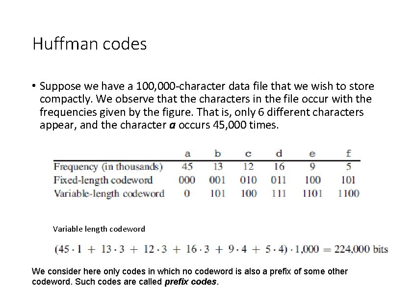
Huffman codes • Suppose we have a 100, 000 -character data file that we wish to store compactly. We observe that the characters in the file occur with the frequencies given by the figure. That is, only 6 different characters appear, and the character a occurs 45, 000 times. Variable length codeword We consider here only codes in which no codeword is also a prefix of some other codeword. Such codes are called prefix codes.

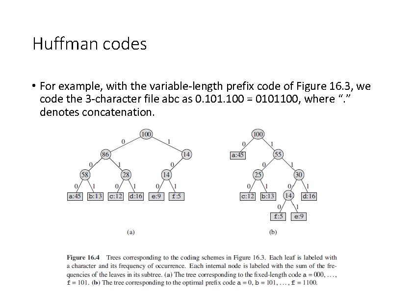
Huffman codes • For example, with the variable-length prefix code of Figure 16. 3, we code the 3 -character file abc as 0. 101. 100 = 0101100, where “. ” denotes concatenation.

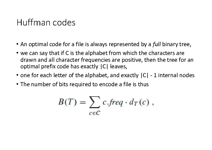
Huffman codes • An optimal code for a file is always represented by a full binary tree, • we can say that if C is the alphabet from which the characters are drawn and all character frequencies are positive, then the tree for an optimal prefix code has exactly |C| leaves, • one for each letter of the alphabet, and exactly |C| - 1 internal nodes • The number of bits required to encode a file is thus

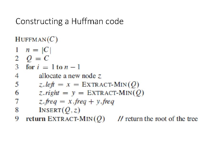
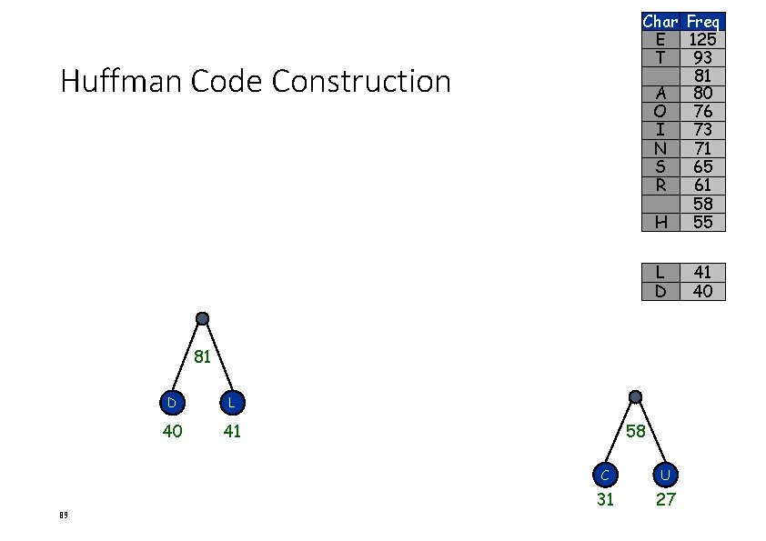
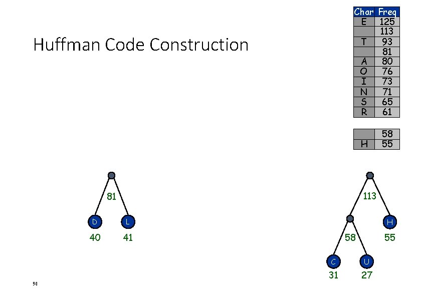
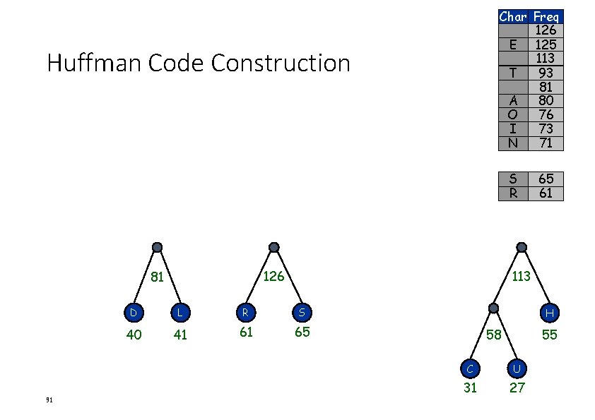
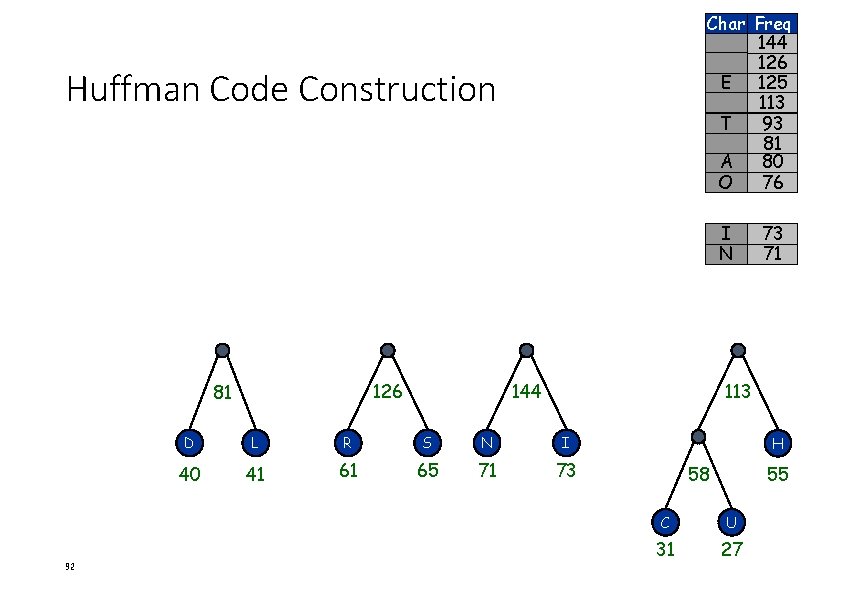
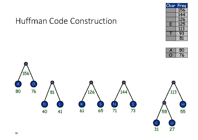
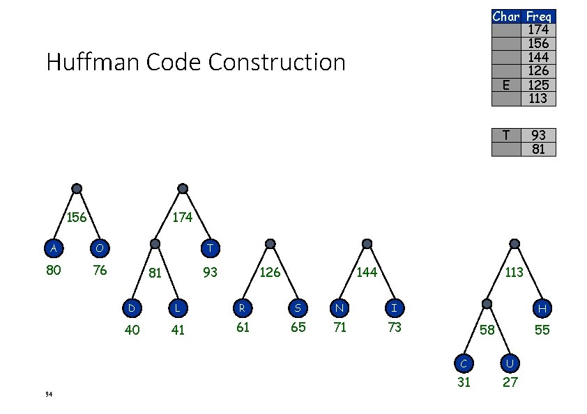
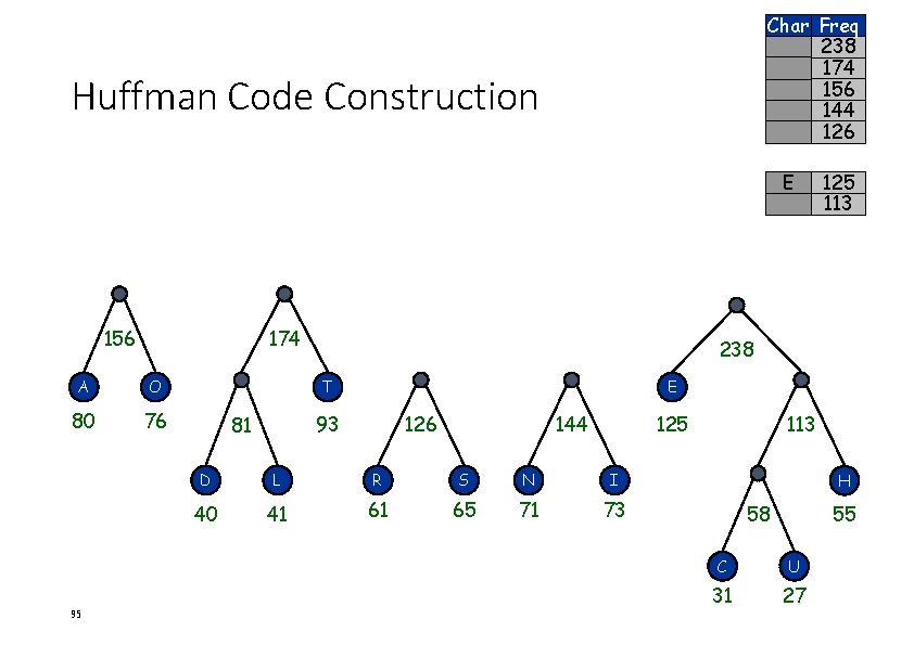
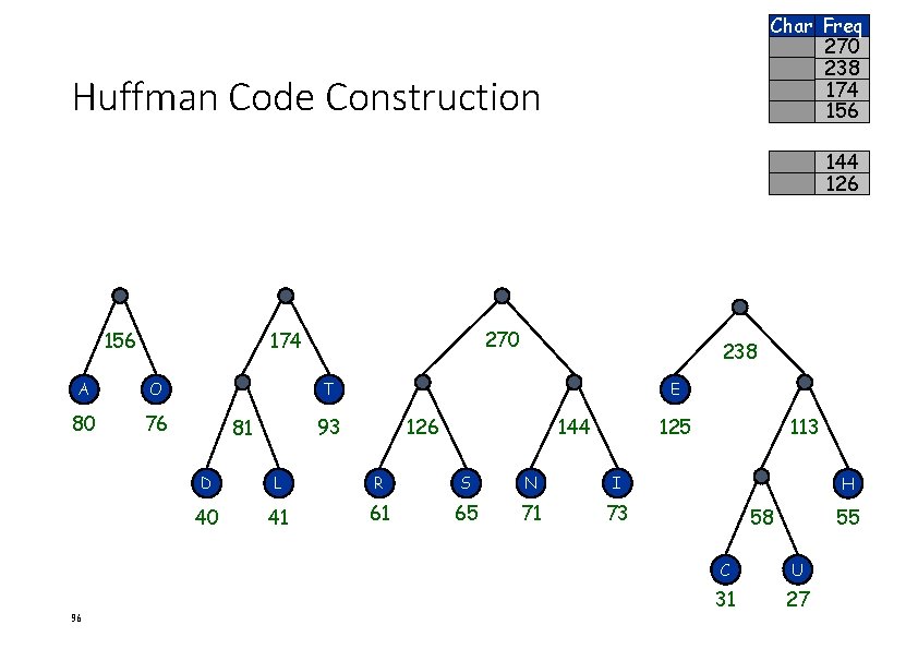
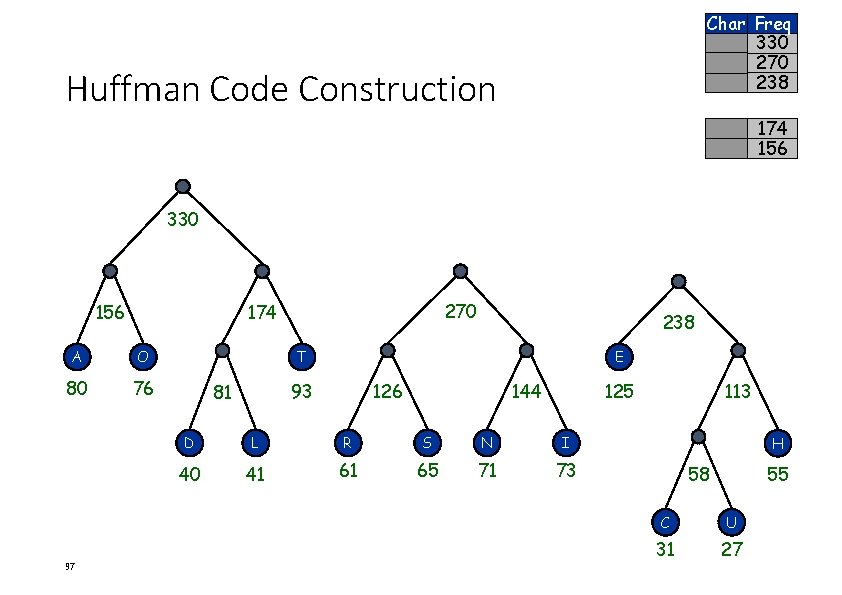
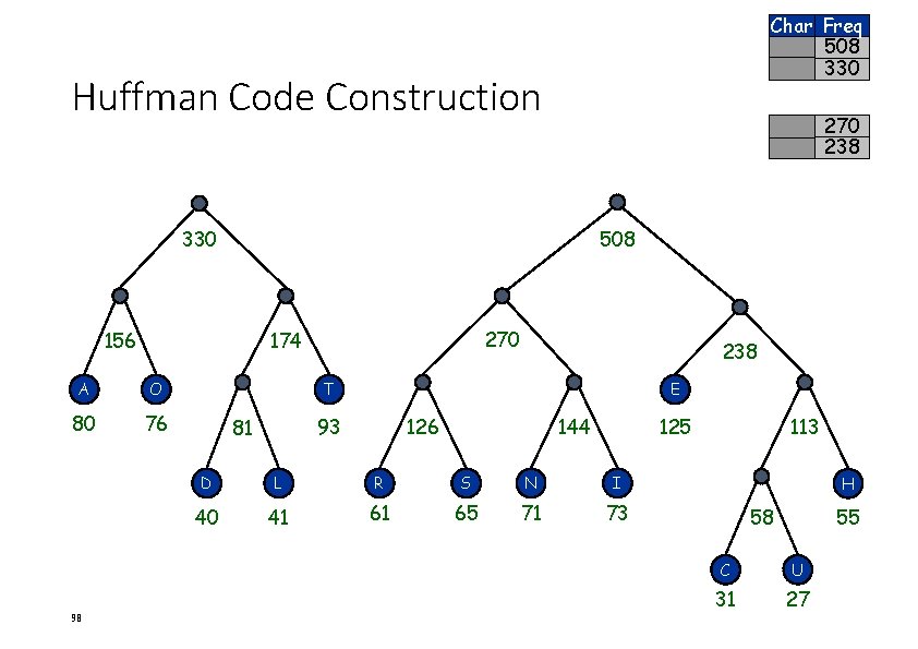
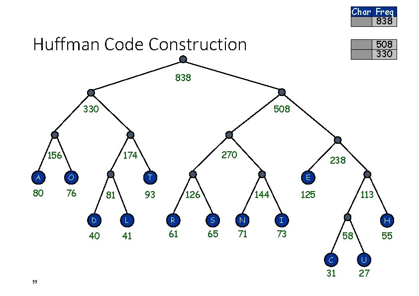
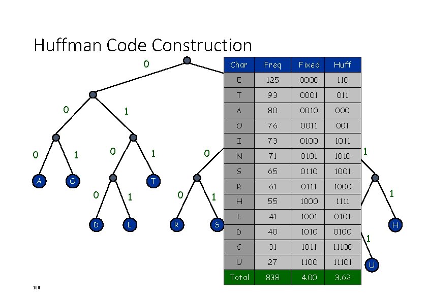
Constructing a Huffman code

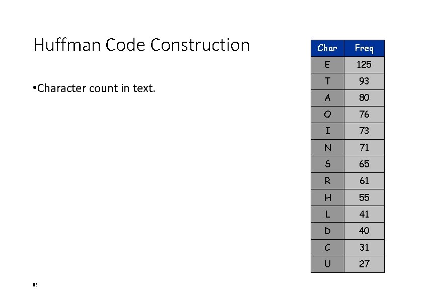
Huffman Code Construction • Character count in text. 86 Char Freq E 125 T 93 A 80 O 76 I 73 N 71 S 65 R 61 H 55 L 41 D 40 C 31 U 27

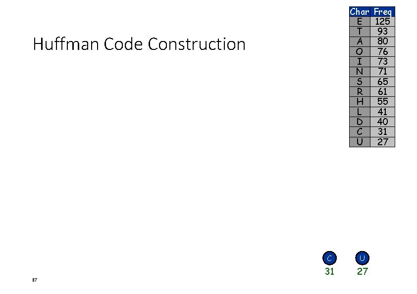
Char E T A O I N S R H L D C U Huffman Code Construction 87 C U 31 27 Freq 125 93 80 76 73 71 65 61 55 41 40 31 27

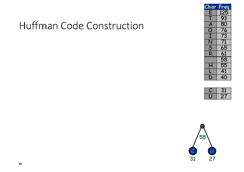
Char E T A O I N S R Huffman Code Construction H L D Freq 125 93 80 76 73 71 65 61 58 55 41 40 C U 31 27 58 88 C U 31 27

Char Freq E 125 T 93 81 A 80 O 76 I 73 N 71 S 65 R 61 58 H 55 Huffman Code Construction L D 81 89 D L 40 41 58 C U 31 27 41 40

Char Freq E 125 113 T 93 81 A 80 O 76 I 73 N 71 S 65 R 61 Huffman Code Construction H 113 81 90 58 55 D L 40 41 H 58 55 C U 31 27

Char Freq 126 E 125 113 T 93 81 A 80 O 76 I 73 N 71 Huffman Code Construction S R 126 81 91 65 61 113 D L R S 40 41 61 65 H 58 55 C U 31 27

Char Freq 144 126 E 125 113 T 93 81 A 80 O 76 Huffman Code Construction I N 126 81 92 144 73 71 113 D L R S N I 40 41 61 65 71 73 H 58 55 C U 31 27

Char Freq 156 144 126 E 125 113 T 93 81 Huffman Code Construction A O 80 76 156 A O 80 76 93 126 81 144 113 D L R S N I 40 41 61 65 71 73 H 58 55 C U 31 27

Char Freq 174 156 144 126 E 125 113 Huffman Code Construction T 156 174 A O 80 76 94 93 81 T 93 81 126 144 113 D L R S N I 40 41 61 65 71 73 H 58 55 C U 31 27

Char Freq 238 174 156 144 126 Huffman Code Construction E 156 174 A O 80 76 95 238 T E 93 81 125 113 126 144 125 D L R S N I 40 41 61 65 71 73 113 H 58 55 C U 31 27

Char Freq 270 238 174 156 Huffman Code Construction 144 126 156 A O 80 76 96 270 174 238 T E 93 81 126 144 125 D L R S N I 40 41 61 65 71 73 113 H 58 55 C U 31 27

Char Freq 330 270 238 Huffman Code Construction 174 156 330 156 A O 80 76 97 270 174 238 T E 93 81 126 144 125 D L R S N I 40 41 61 65 71 73 113 H 58 55 C U 31 27

Char Freq 508 330 Huffman Code Construction 270 238 330 508 156 A O 80 76 98 270 174 238 T E 93 81 126 144 125 D L R S N I 40 41 61 65 71 73 113 H 58 55 C U 31 27

Char Freq 838 Huffman Code Construction 508 330 838 330 508 156 A O 80 76 99 270 174 238 T E 93 81 126 144 125 D L R S N I 40 41 61 65 71 73 113 H 58 55 C U 31 27

Huffman Code Construction 0 0 0 A 0 D 100 0 T 0 1 L Fixed Huff E 125 0000 110 T 93 0001 011 80 0010 1 000 O 76 0011 001 I 73 0100 1011 0101 0 1010 0110 E 0111 1000 1111 1001 0101 1010 0100 A 1 O Freq 1 1 1 Char 0 R 1 S 0 N 1 71 S 65 R 61 H L D 0 N 55 41 40 1 I 0 1 1 0 C 31 1011 11100 U 27 1100 11101 C Total 838 4. 00 3. 62 H 1 U

Correctness of Huffman’s algorithm Proof Idea • Step 1: Show that this problem satisfies the greedy choice property, that is, if a greedy choice is made by Huffman's algorithm, an optimal solution remains possible. • Step 2: Show that this problem has an optimal substructure property, that is, an optimal solution to Huffman's algorithm contains optimal solution to subproblems. • Step 3: Conclude correctness of Huffman's algorithm using step 1 and step 2.

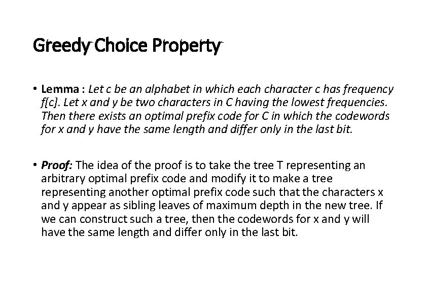
Greedy Choice Property • Lemma : Let c be an alphabet in which each character c has frequency f[c]. Let x and y be two characters in C having the lowest frequencies. Then there exists an optimal prefix code for C in which the codewords for x and y have the same length and differ only in the last bit. • Proof: The idea of the proof is to take the tree T representing an arbitrary optimal prefix code and modify it to make a tree representing another optimal prefix code such that the characters x and y appear as sibling leaves of maximum depth in the new tree. If we can construct such a tree, then the codewords for x and y will have the same length and differ only in the last bit.

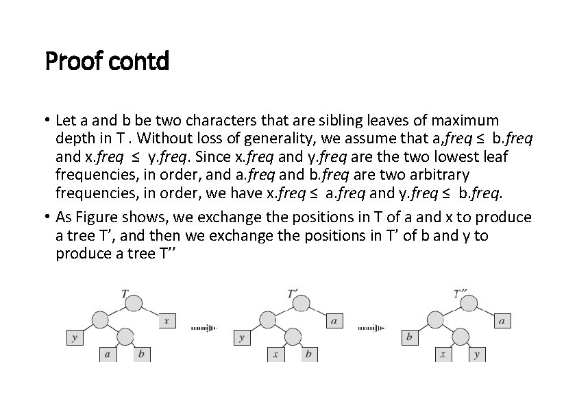
Proof contd • Let a and b be two characters that are sibling leaves of maximum depth in T. Without loss of generality, we assume that a, freq ≤ b. freq and x. freq ≤ y. freq. Since x. freq and y. freq are the two lowest leaf frequencies, in order, and a. freq and b. freq are two arbitrary frequencies, in order, we have x. freq ≤ a. freq and y. freq ≤ b. freq. • As Figure shows, we exchange the positions in T of a and x to produce a tree T’, and then we exchange the positions in T’ of b and y to produce a tree T’’

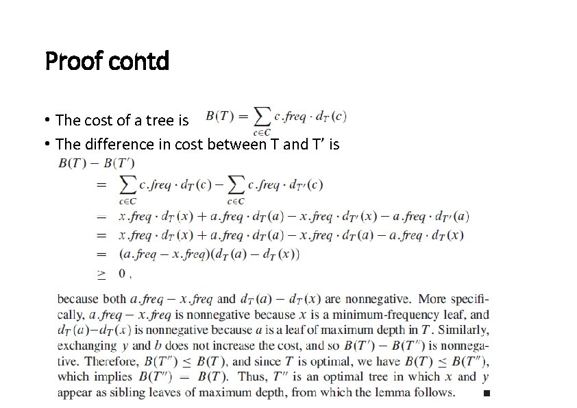
Proof contd • The cost of a tree is • The difference in cost between T and T’ is

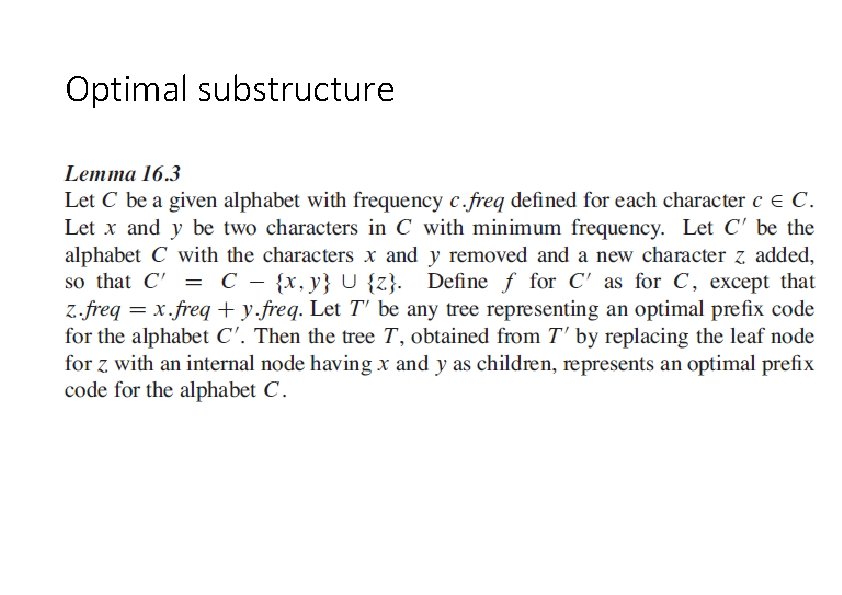
Optimal substructure

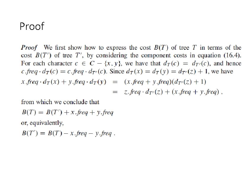
Proof

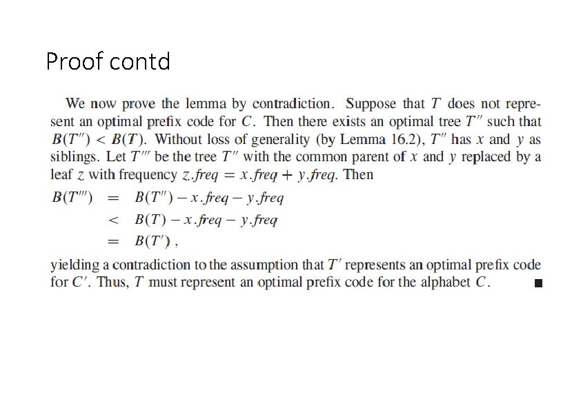
Proof contd