Chapter One Introduction to Pipelined Processors Principle of

Chapter One Introduction to Pipelined Processors

Principle of Designing Pipeline Processors (Design Problems of Pipeline Processors)

Job Sequencing and Collision Prevention

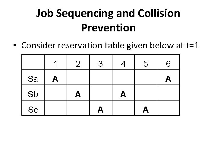
Job Sequencing and Collision Prevention • Consider reservation table given below at t=1 1 Sa A Sb Sc 2 3 4 5 6 A A A

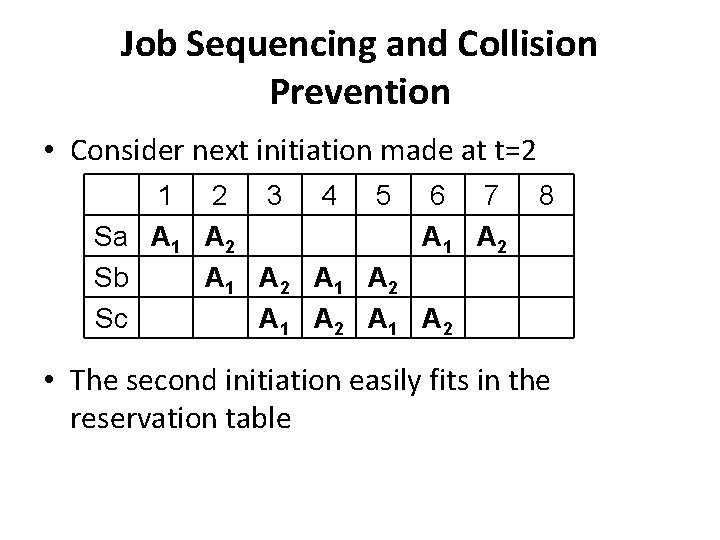
Job Sequencing and Collision Prevention • Consider next initiation made at t=2 1 2 3 4 5 6 7 Sa A 1 A 2 Sb A 1 A 2 Sc A 1 A 2 8 • The second initiation easily fits in the reservation table

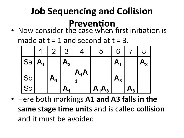
Job Sequencing and Collision Prevention • Now consider the case when first initiation is made at t = 1 and second at t = 3. 1 2 3 Sa A 1 A 3 Sb Sc 4 5 A 1 A A 1 A 3 3 A 1 6 7 8 A 1 A 3 A 1 A 3 • Here both markings A 1 and A 3 falls in the same stage time units and is called collision and it must be avoided

Terminologies

Terminologies • Latency: Time difference between two initiations in units of clock period • Forbidden Latency: Latencies resulting in collision • Forbidden Latency Set: Set of all forbidden latencies

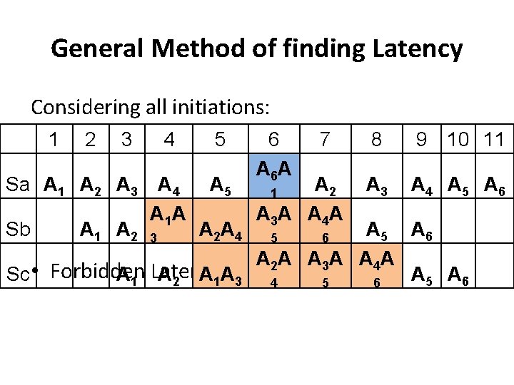
General Method of finding Latency Considering all initiations: 1 2 3 Sa A 1 A 2 A 3 Sb A 1 A 2 4 5 A 4 A 1 A A 5 7 A 2 A 3 A A 4 A 1 8 9 10 11 A 3 A 4 A 5 A 6 A 2 A A 3 A A 4 A Sc • Forbidden A 1 Latencies A 2 A 1 A 3 are 42 and 5 5 6 A 5 A 6 3 A 2 A 4 6 A 6 A 5 6

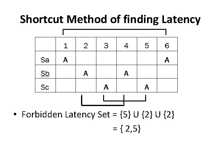
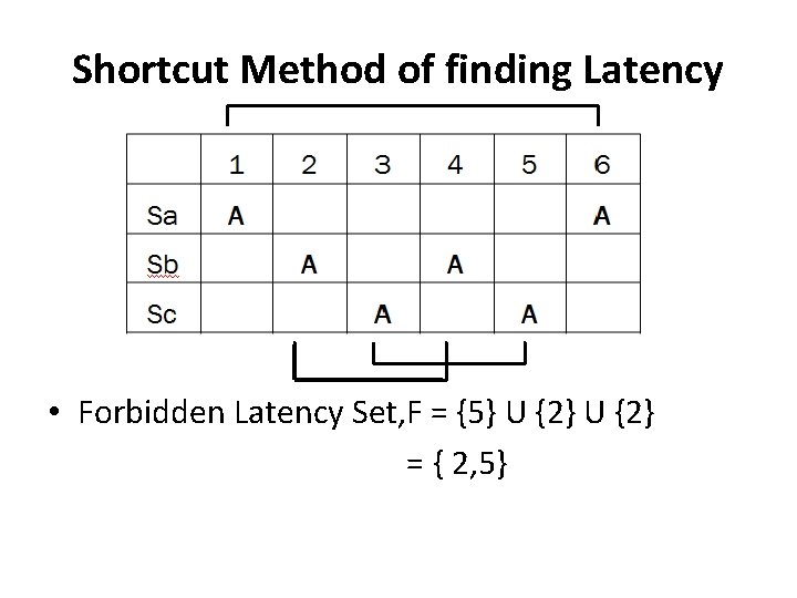
Shortcut Method of finding Latency • Forbidden Latency Set = {5} U {2} = { 2, 5}

Terminologies • Latency Sequence : Sequence of latencies between successive initiations • For a RT, number of valid initiations and latencies are infinite

Terminologies • Latency Cycle: • Among the infinite possible latency sequence, the periodic ones are significant. E. g. { 1, 3, 3, … } • The subsequence that repeats itself is called latency cycle. E. g. {1, 3, 3}

Terminologies • Period of cycle: The sum of latencies in a latency cycle (1+3+3=7) • Average Latency: The average taken over its latency cycle (AL=7/3=2. 33) • To design a pipeline, we need a control strategy that maximize throughput (no. of results per unit time) • Maximizing throughput is minimizing AL

Terminologies • Latency sequence which is aperiodic in nature is impossible to design • Thus design problem is arriving at a latency cycle having minimal average latency.

State Diagram

Shortcut Method of finding Latency • Forbidden Latency Set, F = {5} U {2} = { 2, 5}

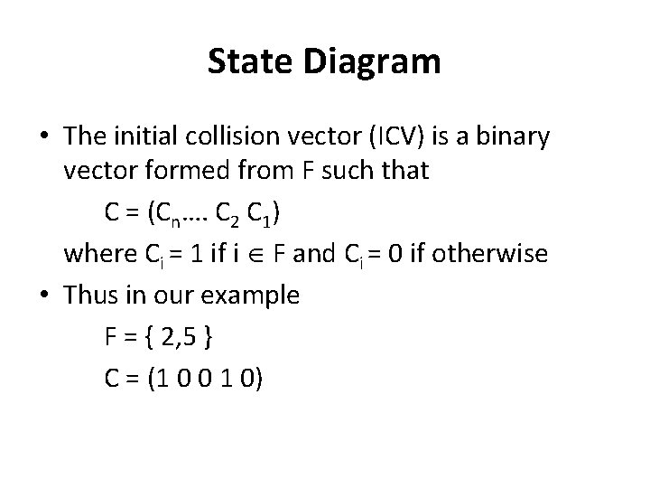
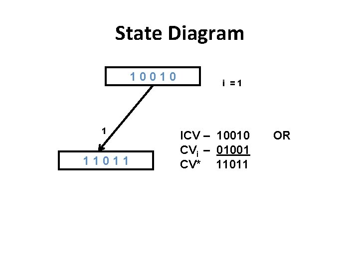
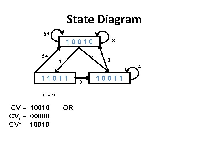
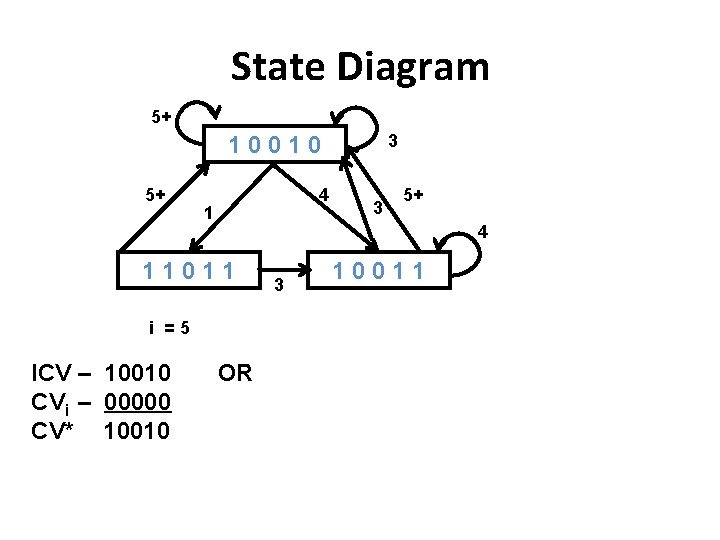
State Diagram • The initial collision vector (ICV) is a binary vector formed from F such that C = (Cn…. C 2 C 1) where Ci = 1 if i F and Ci = 0 if otherwise • Thus in our example F = { 2, 5 } C = (1 0 0 1 0)

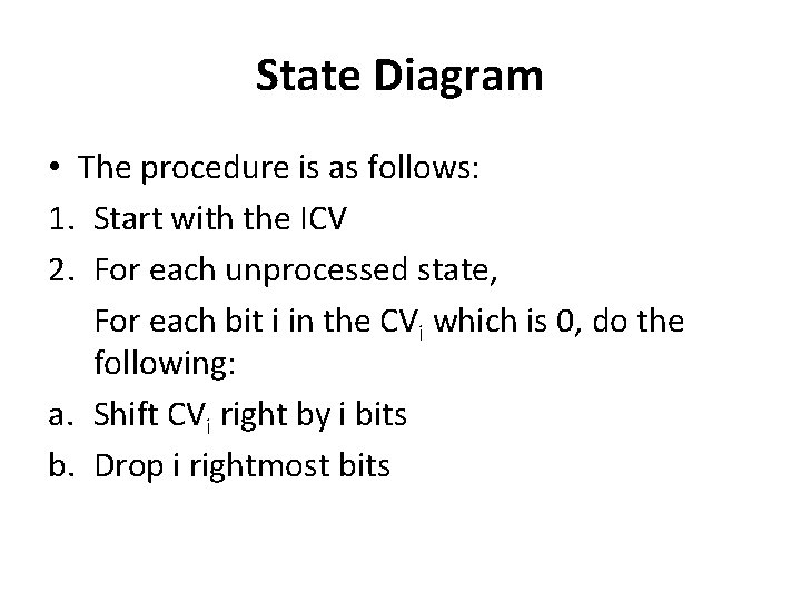
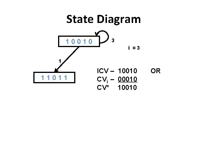
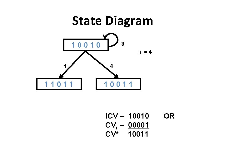
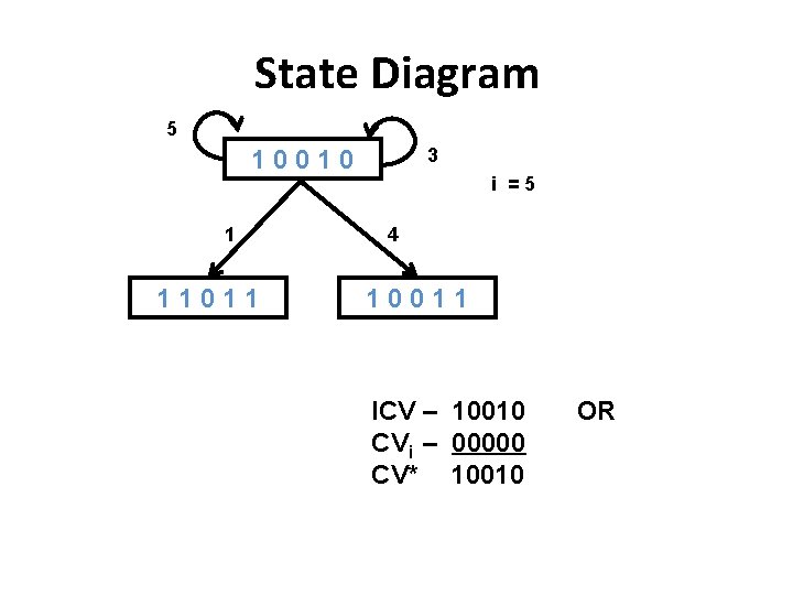
State Diagram • The procedure is as follows: 1. Start with the ICV 2. For each unprocessed state, For each bit i in the CVi which is 0, do the following: a. Shift CVi right by i bits b. Drop i rightmost bits

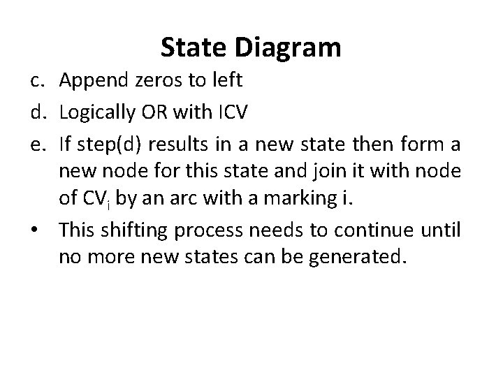
State Diagram c. Append zeros to left d. Logically OR with ICV e. If step(d) results in a new state then form a new node for this state and join it with node of CVi by an arc with a marking i. • This shifting process needs to continue until no more new states can be generated.

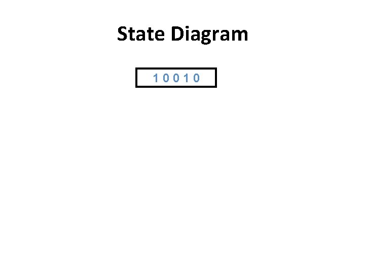
State Diagram 10010

State Diagram 10010 1 11011 i =1 ICV – 10010 CVi – 01001 CV* 11011 OR

State Diagram 10010 3 i =3 1 11011 ICV – 10010 CVi – 00010 CV* 10010 OR

State Diagram 3 10010 1 11011 i =4 4 10011 ICV – 10010 CVi – 00001 CV* 10011 OR

State Diagram 5 3 10010 1 11011 i =5 4 10011 ICV – 10010 CVi – 00000 CV* 10010 OR

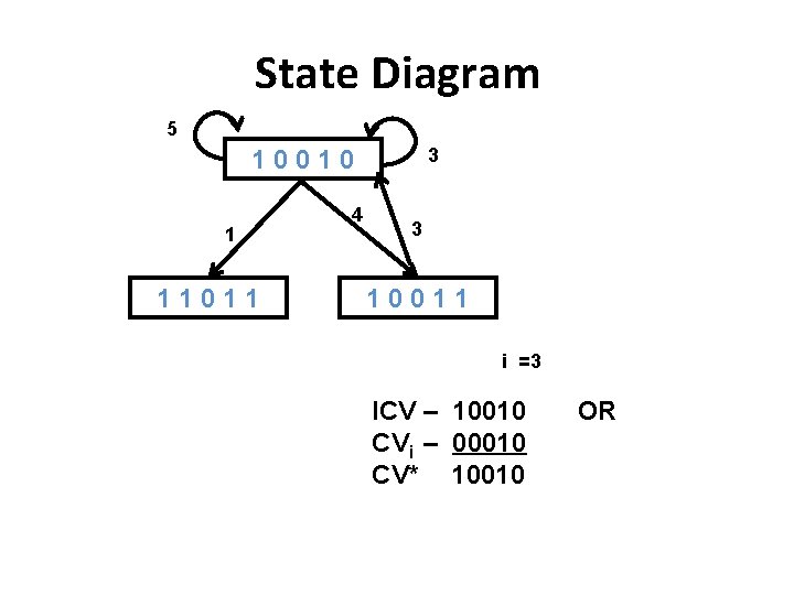
State Diagram 5 3 10010 1 11011 4 3 10011 i =3 ICV – 10010 CVi – 00010 CV* 10010 OR

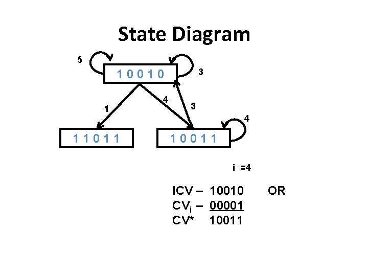
State Diagram 5 3 10010 1 11011 4 3 4 10011 i =4 ICV – 10010 CVi – 00001 CV* 10011 OR

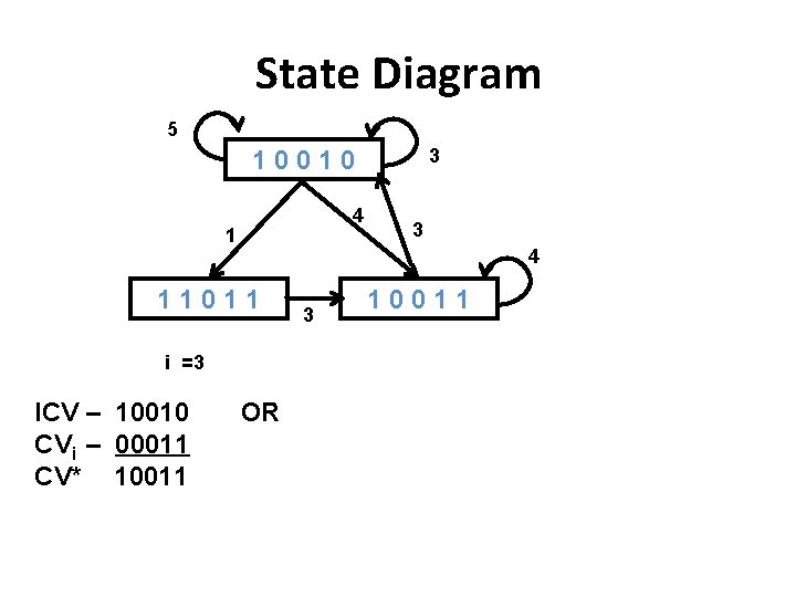
State Diagram 5 3 10010 4 11011 i =3 ICV – 10010 CVi – 00011 CV* 10011 3 OR 3 10011

State Diagram 5+ 3 10010 5+ 4 11011 i =5 ICV – 10010 CVi – 00000 CV* 10010 3 OR 3 10011

State Diagram 5+ 3 10010 5+ 4 11011 i =5 ICV – 10010 CVi – 00000 CV* 10010 3 OR 3 10011

State Diagram • The state with all zeros has a self-loop which corresponds to empty pipeline and it is possible to wait for indefinite number of latency cycles of the form (7), (8), (9), (10) etc. • Simple Cycle: latency cycle in which each state is encountered only once. • Complex Cycle: consists of more than one simple cycle in it. • It is enough to look for simple cycles

State Diagram • Greedy Cycle: A simple cycle is a greedy cycle if each latency contained in a cycle is the minimal latency(outgoing arc) from a state in the cycle. • A good task initiation sequence should include the greedy cycle.

Simple cycles & Greedy cycles • The Simple cycles are? • The Greedy cycles are ?

Simple cycles & Greedy cycles • The simple cycles are (3), (5) , (1, 3, 3), (4, 3) and (4) • The Greedy cycle is (1, 3, 3)

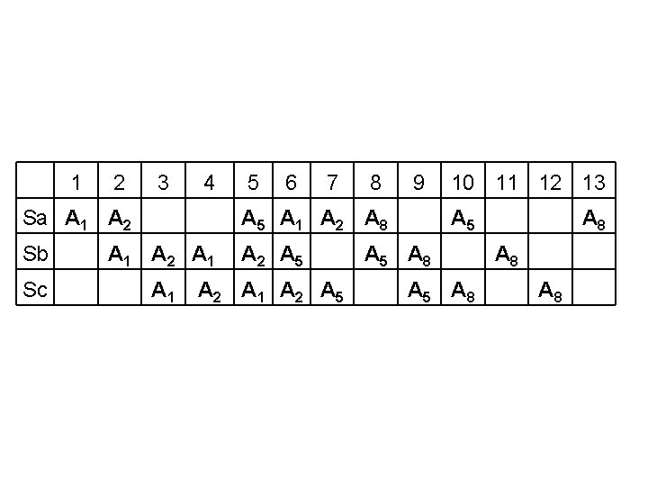
State Diagram • In the above example, the cycle that offers MAL is (1, 3, 3) (MAL = (1+3+3)/3 =2. 333)

1 2 3 4 5 6 7 8 Sa A 1 A 2 A 5 A 1 A 2 A 8 Sb A 1 A 2 A 5 Sc A 1 A 2 A 5 9 10 11 12 13 A 5 A 8 A 8

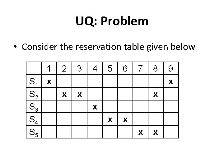
UQ: Problem • Consider the reservation table given below 1 S 1 x S 2 S 3 S 4 S 5 2 3 x x 4 5 6 7 8 x x x 9 x

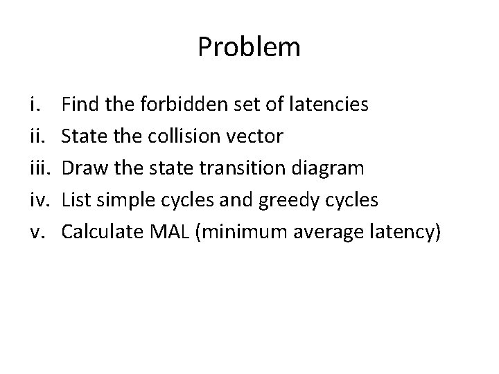
Problem i. iii. iv. v. Find the forbidden set of latencies State the collision vector Draw the state transition diagram List simple cycles and greedy cycles Calculate MAL (minimum average latency)