Greedy Algorithms TOPICS Greedy Strategy Activity Selection Chapter

Greedy Algorithms TOPICS • Greedy Strategy • Activity Selection Chapter 5 • Minimum Spanning Tree Algorithm Design Kleinberg and Tardos • Shortest Paths • Huffman Codes • Fractional Knapsack 10/22/2021 CSE 5311 Spring 2007 M Kumar 1

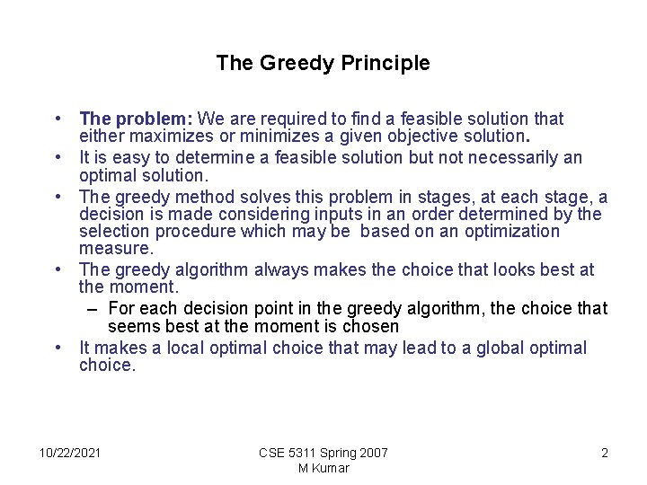
The Greedy Principle • The problem: We are required to find a feasible solution that either maximizes or minimizes a given objective solution. • It is easy to determine a feasible solution but not necessarily an optimal solution. • The greedy method solves this problem in stages, at each stage, a decision is made considering inputs in an order determined by the selection procedure which may be based on an optimization measure. • The greedy algorithm always makes the choice that looks best at the moment. – For each decision point in the greedy algorithm, the choice that seems best at the moment is chosen • It makes a local optimal choice that may lead to a global optimal choice. 10/22/2021 CSE 5311 Spring 2007 M Kumar 2

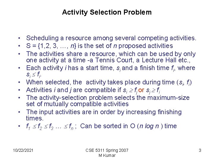
Activity Selection Problem • Scheduling a resource among several competing activities. • S = {1, 2, 3, …, n} is the set of n proposed activities • The activities share a resource, which can be used by only one activity at a time -a Tennis Court, a Lecture Hall etc. , • Each activity i has a start time, si and a finish time fi, where si fi. • When selected, the activity takes place during time (si, fi) • Activities i and j are compatible if si fj or sj fi • The activity-selection problem selects the maximum-size set of mutually compatible activities • The input activities are in order by increasing finishing times. • f 1 f 2 f 3 … fn ; Can be sorted in O (n log n ) time 10/22/2021 CSE 5311 Spring 2007 M Kumar 3

Procedure for activity selection (from CLRS) Procedure GREEDY_ACTIVITY_SELECTOR(s, f) n length [S]; in order of increasing finishing times; A {1}; first job to finish j 1; for i 2 to n do if si fj then A A {i}; j i; 10/22/2021 CSE 5311 Spring 2007 M Kumar 4

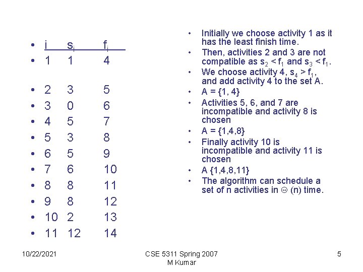
• i • 1 si 1 fi 4 • • • 3 0 5 3 5 6 8 8 2 12 5 6 7 8 9 10 11 12 13 14 2 3 4 5 6 7 8 9 10 11 10/22/2021 • • • Initially we choose activity 1 as it has the least finish time. Then, activities 2 and 3 are not compatible as s 2 < f 1 and s 3 < f 1. We choose activity 4, s 4 > f 1, and add activity 4 to the set A. A = {1, 4} Activities 5, 6, and 7 are incompatible and activity 8 is chosen A = {1, 4, 8} Finally activity 10 is incompatible and activity 11 is chosen A {1, 4, 8, 11} The algorithm can schedule a set of n activities in (n) time. CSE 5311 Spring 2007 M Kumar 5

Minimum-Cost Spanning Trees Consider a network of computers connected through bidirectional links. Each link is associated with a positive cost: the cost of sending a message on each link. This network can be represented by an undirected graph with positive costs on each edge. In bidirectional networks we can assume that the cost of sending a message on a link does not depend on the direction. Suppose we want to broadcast a message to all the computers from an arbitrary computer. The cost of the broadcast is the sum of the costs of links used to forward the message. 10/22/2021 CSE 5311 Spring 2007 M Kumar 6

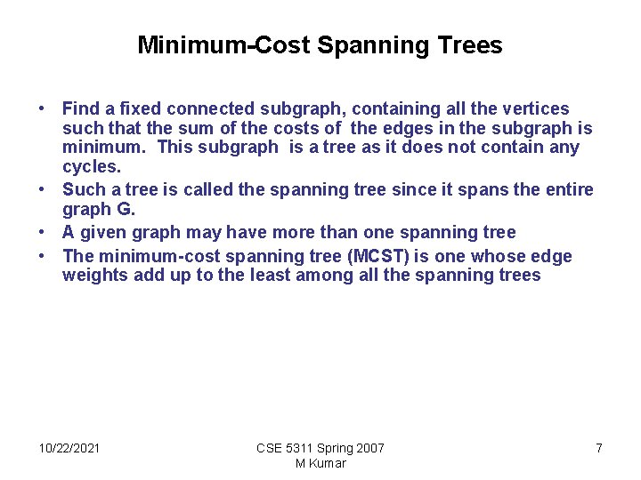
Minimum-Cost Spanning Trees • Find a fixed connected subgraph, containing all the vertices such that the sum of the costs of the edges in the subgraph is minimum. This subgraph is a tree as it does not contain any cycles. • Such a tree is called the spanning tree since it spans the entire graph G. • A given graph may have more than one spanning tree • The minimum-cost spanning tree (MCST) is one whose edge weights add up to the least among all the spanning trees 10/22/2021 CSE 5311 Spring 2007 M Kumar 7

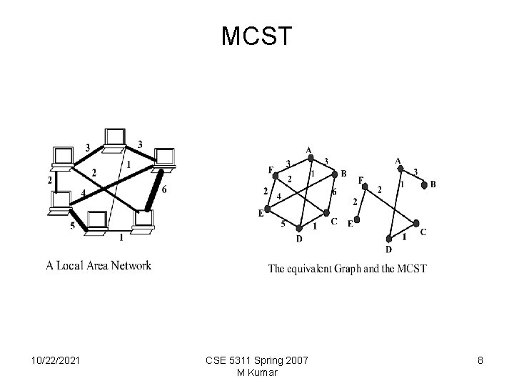
MCST 10/22/2021 CSE 5311 Spring 2007 M Kumar 8

MCST • The Problem: Given an undirected connected weighted graph G =(V, E), find a spanning tree T of G of minimum cost. • Greedy Algorithm for finding the Minimum Spanning Tree of a Graph G =(V, E) The algorithm is also called Kruskal's algorithm. • At each step of the algorithm, one of several possible choices must be made, • The greedy strategy: make the choice that is the best at the moment 10/22/2021 CSE 5311 Spring 2007 M Kumar 9

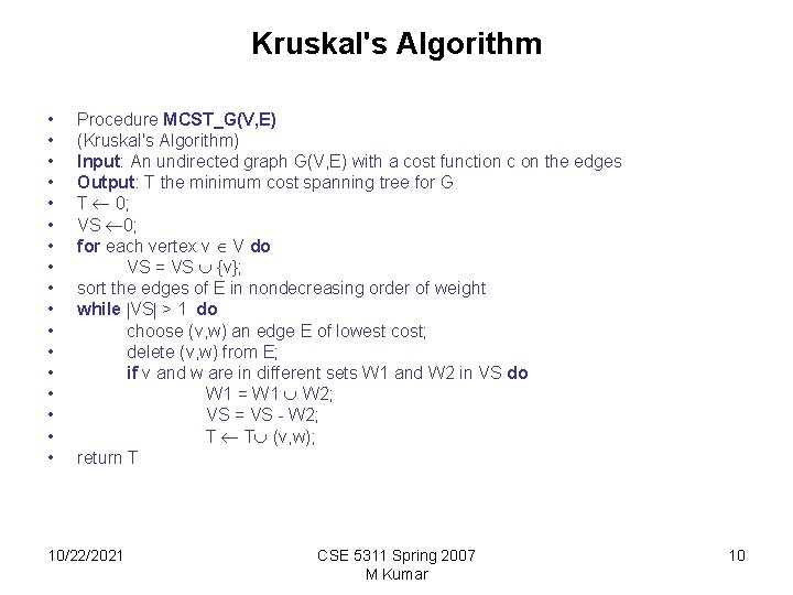
Kruskal's Algorithm • • • • • Procedure MCST_G(V, E) (Kruskal's Algorithm) Input: An undirected graph G(V, E) with a cost function c on the edges Output: T the minimum cost spanning tree for G T 0; VS 0; for each vertex v V do VS = VS {v}; sort the edges of E in nondecreasing order of weight while VS > 1 do choose (v, w) an edge E of lowest cost; delete (v, w) from E; if v and w are in different sets W 1 and W 2 in VS do W 1 = W 1 W 2; VS = VS - W 2; T T (v, w); return T 10/22/2021 CSE 5311 Spring 2007 M Kumar 10

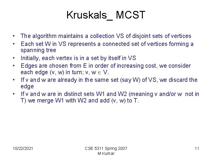
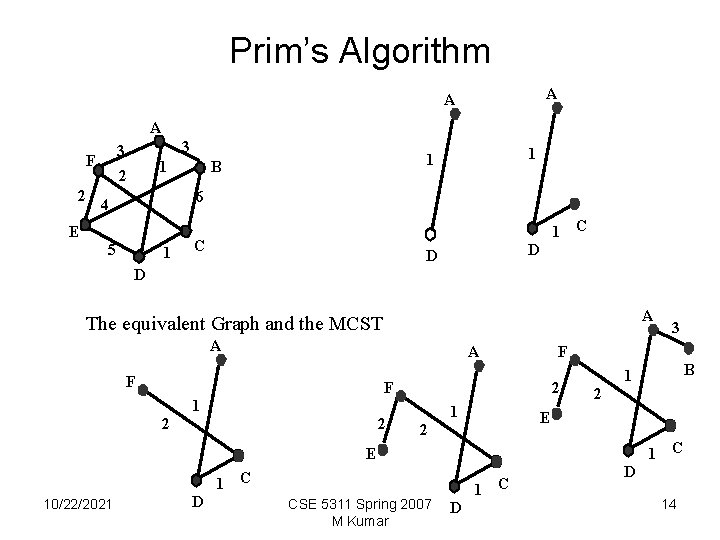
Kruskals_ MCST • The algorithm maintains a collection VS of disjoint sets of vertices • Each set W in VS represents a connected set of vertices forming a spanning tree • Initially, each vertex is in a set by itself in VS • Edges are chosen from E in order of increasing cost, we consider each edge (v, w) in turn; v, w V. • If v and w are already in the same set (say W) of VS, we discard the edge • If v and w are in distinct sets W 1 and W 2 (meaning v and/or w not in T) we merge W 1 with W 2 and add (v, w) to T. 10/22/2021 CSE 5311 Spring 2007 M Kumar 11

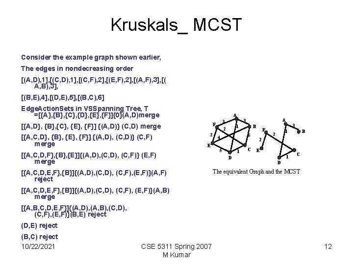
Kruskals_ MCST Consider the example graph shown earlier, The edges in nondecreasing order [(A, D), 1], [(C, F), 2], [(E, F), 2], [(A, F), 3], [( A, B), 3], [(B, E), 4], [(D, E), 5], [(B, C), 6] Edge. Action. Sets in VSSpanning Tree, T =[{A}, {B}, {C}, {D}, {E}, {F}]{0}(A, D)merge A [{A, C, D}, {B}, {E}, {F}] {(A, D), (C, D)} (C, F) merge 2 E [{A, C, D, F}, {B}, {E}]{(A, D), (C, F)} (E, F) merge [{A, C, D, E, F}, {B}]{(A, D), (C, F), (E, F)}(A, F) reject A 3 3 2 F [{A, D}, {B}, {C}, {E}, {F}] {(A, D)} (C, D) merge 1 B 6 4 5 1 D C F 3 1 2 B 2 E 1 C D The equivalent Graph and the MCST [{A, C, D, E, F}, {B}]{(A, D), (C, F), (E, F)}(A, B) merge [{A, B, C, D, E, F}]{(A, D), (A, B), (C, D), (C, F), (E, F)}(B, E) reject (D, E) reject (B, C) reject 10/22/2021 CSE 5311 Spring 2007 M Kumar 12

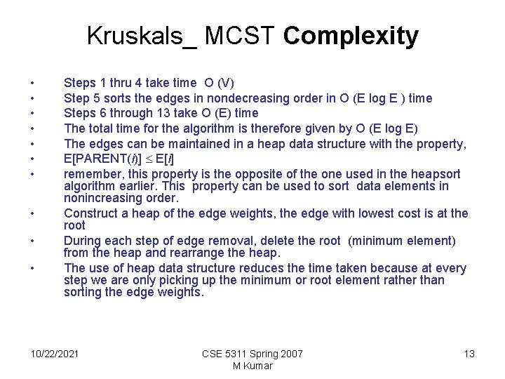
Kruskals_ MCST Complexity • • • Steps 1 thru 4 take time O (V) Step 5 sorts the edges in nondecreasing order in O (E log E ) time Steps 6 through 13 take O (E) time The total time for the algorithm is therefore given by O (E log E) The edges can be maintained in a heap data structure with the property, E[PARENT(i)] E[i] remember, this property is the opposite of the one used in the heapsort algorithm earlier. This property can be used to sort data elements in nonincreasing order. Construct a heap of the edge weights, the edge with lowest cost is at the root During each step of edge removal, delete the root (minimum element) from the heap and rearrange the heap. The use of heap data structure reduces the time taken because at every step we are only picking up the minimum or root element rather than sorting the edge weights. 10/22/2021 CSE 5311 Spring 2007 M Kumar 13

Prim’s Algorithm A A A 2 E 3 3 F 1 2 1 1 B 6 4 5 1 1 C C D D D A The equivalent Graph and the MCST A A F F 2 F 1 2 2 1 2 E 2 1 C D CSE 5311 Spring 2007 M Kumar B 1 E 10/22/2021 3 1 C D D 14

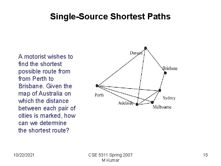
Single-Source Shortest Paths A motorist wishes to find the shortest possible route from Perth to Brisbane. Given the map of Australia on which the distance between each pair of cities is marked, how can we determine the shortest route? 10/22/2021 CSE 5311 Spring 2007 M Kumar 15

Single Source Shortest Path • In a shortest-paths problem, we are given a weighted, directed graph G = (V, E), with weights assigned to each edge in the graph. The weight of the path p = (v 0, v 1, v 2, …, vk) is the sum of the weights of its constituent edges: • v 0 v 1 v 2. . . vk-1 vk • • The shortest-path from u to v is given by • d(u, v) = min {weight (p) : if there are one or more paths from u to v • = otherwise 10/22/2021 CSE 5311 Spring 2007 M Kumar 16

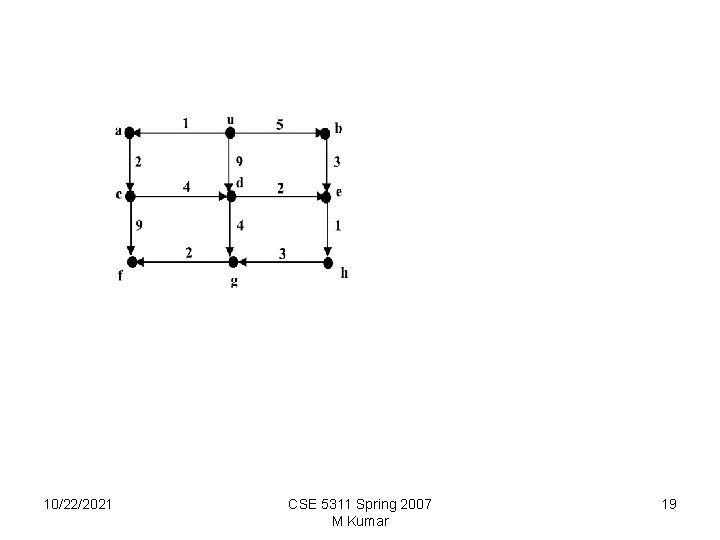
The single-source shortest paths problem Given G (V, E), find the shortest path from a given vertex u V to every vertex v V ( u v). For each vertex v V in the weighted directed graph, d[v] represents the distance from u to v. Initially, d[v] = 0 when u = v. d[v] = if (u, v) is not an edge d[v] = weight of edge (u, v) if (u, v) exists. Dijkstra's Algorithm : At every step of the algorithm, we compute, d[y] = min {d[y], d[x] + w(x, y)}, where x, y V. Dijkstra's algorithm is based on the greedy principle because at every step we pick the path of least weight. 10/22/2021 CSE 5311 Spring 2007 M Kumar 17

• Dijkstra's Algorithm : At every step of the algorithm, we compute, d[y] = min {d[y], d[x] + w(x, y)}, where x, y V. • Dijkstra's algorithm is based on the greedy principle because at every step we pick the path of least path. 10/22/2021 CSE 5311 Spring 2007 M Kumar 18

10/22/2021 CSE 5311 Spring 2007 M Kumar 19

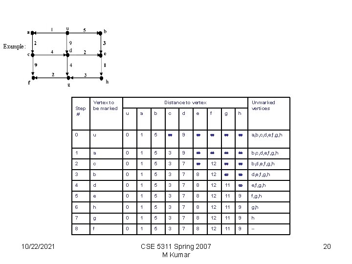
Example: Step # 10/22/2021 Vertex to be marked Distance to vertex u a b c d e f g h Unmarked vertices 0 u 0 1 5 9 a, b, c, d, e, f, g, h 1 a 0 1 5 3 9 b, c, d, e, f, g, h 2 c 0 1 5 3 7 12 b, d, e, f, g, h 3 b 0 1 5 3 7 8 12 d, e, f, g, h 4 d 0 1 5 3 7 8 12 11 e, f, g, h 5 e 0 1 5 3 7 8 12 11 9 f, g, h 6 h 0 1 5 3 7 8 12 11 9 g, h 7 g 0 1 5 3 7 8 12 11 9 h 8 f 0 1 5 3 7 8 12 11 9 -- CSE 5311 Spring 2007 M Kumar 20

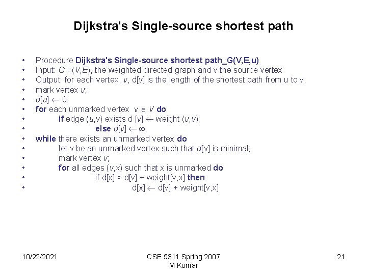
Dijkstra's Single-source shortest path • • • • Procedure Dijkstra's Single-source shortest path_G(V, E, u) Input: G =(V, E), the weighted directed graph and v the source vertex Output: for each vertex, v, d[v] is the length of the shortest path from u to v. mark vertex u; d[u] 0; for each unmarked vertex v V do if edge (u, v) exists d [v] weight (u, v); else d[v] ; while there exists an unmarked vertex do let v be an unmarked vertex such that d[v] is minimal; mark vertex v; for all edges (v, x) such that x is unmarked do if d[x] > d[v] + weight[v, x] then d[x] d[v] + weight[v, x] 10/22/2021 CSE 5311 Spring 2007 M Kumar 21

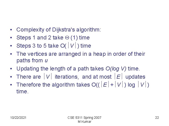
• • Complexity of Dijkstra's algorithm: Steps 1 and 2 take (1) time Steps 3 to 5 take O( V ) time The vertices are arranged in a heap in order of their paths from u • Updating the length of a path takes O(log V) time. • There are V iterations, and at most E updates • Therefore the algorithm takes O(( E + V ) log V ) time. 10/22/2021 CSE 5311 Spring 2007 M Kumar 22

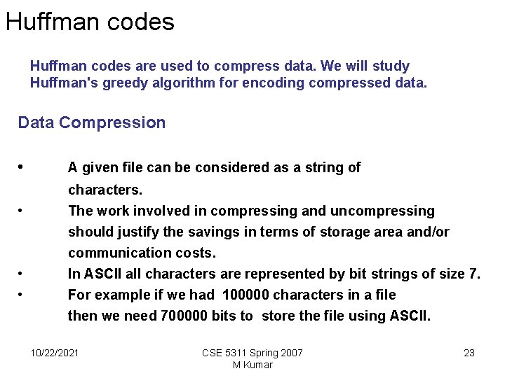
Huffman codes are used to compress data. We will study Huffman's greedy algorithm for encoding compressed data. Data Compression • A given file can be considered as a string of • characters. The work involved in compressing and uncompressing • • should justify the savings in terms of storage area and/or communication costs. In ASCII all characters are represented by bit strings of size 7. For example if we had 100000 characters in a file then we need 700000 bits to store the file using ASCII. 10/22/2021 CSE 5311 Spring 2007 M Kumar 23

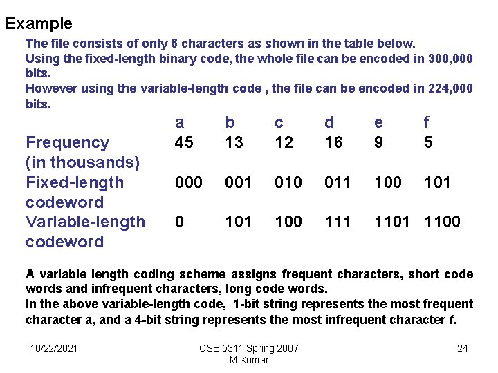
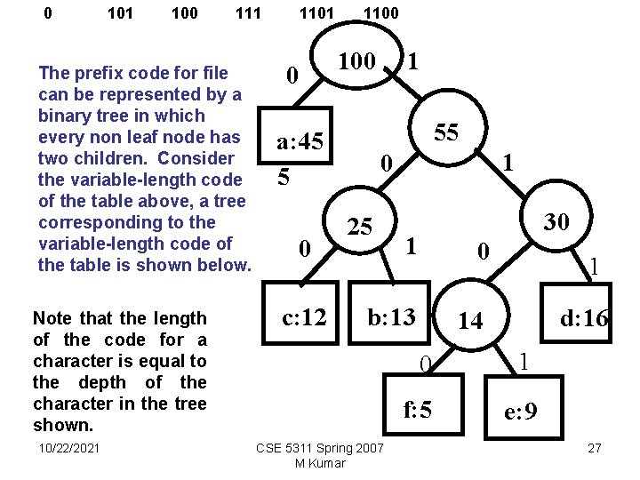
Example The file consists of only 6 characters as shown in the table below. Using the fixed-length binary code, the whole file can be encoded in 300, 000 bits. However using the variable-length code , the file can be encoded in 224, 000 bits. Frequency (in thousands) Fixed-length codeword Variable-length codeword a 45 b 13 c 12 d 16 e 9 f 5 000 001 010 011 100 101 100 111 1100 A variable length coding scheme assigns frequent characters, short code words and infrequent characters, long code words. In the above variable-length code, 1 -bit string represents the most frequent character a, and a 4 -bit string represents the most infrequent character f. 10/22/2021 CSE 5311 Spring 2007 M Kumar 24

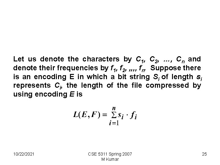
Let us denote the characters by C 1, C 2, …, Cn and denote their frequencies by f 1, f 2, , , fn. Suppose there is an encoding E in which a bit string Si of length si represents Ci, the length of the file compressed by using encoding E is 10/22/2021 CSE 5311 Spring 2007 M Kumar 25

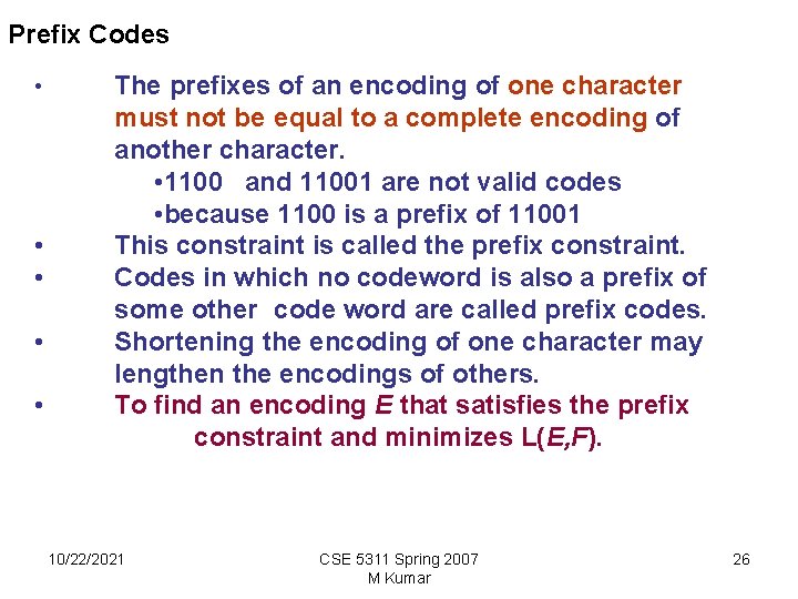
Prefix Codes • • • The prefixes of an encoding of one character must not be equal to a complete encoding of another character. • 1100 and 11001 are not valid codes • because 1100 is a prefix of 11001 This constraint is called the prefix constraint. Codes in which no codeword is also a prefix of some other code word are called prefix codes. Shortening the encoding of one character may lengthen the encodings of others. To find an encoding E that satisfies the prefix constraint and minimizes L(E, F). 10/22/2021 CSE 5311 Spring 2007 M Kumar 26

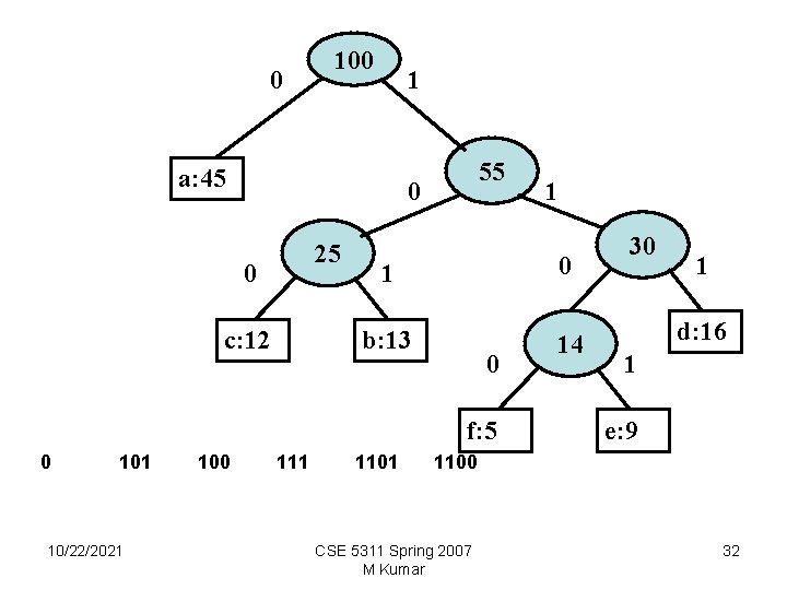
0 101 100 111 The prefix code for file can be represented by a binary tree in which every non leaf node has two children. Consider the variable-length code of the table above, a tree corresponding to the variable-length code of the table is shown below. Note that the length of the code for a character is equal to the depth of the character in the tree shown. 10/22/2021 1100 1 100 0 55 a: 45 5 0 c: 12 1 0 25 30 1 0 b: 13 14 CSE 5311 Spring 2007 M Kumar 1 d: 16 0 1 f: 5 e: 9 27

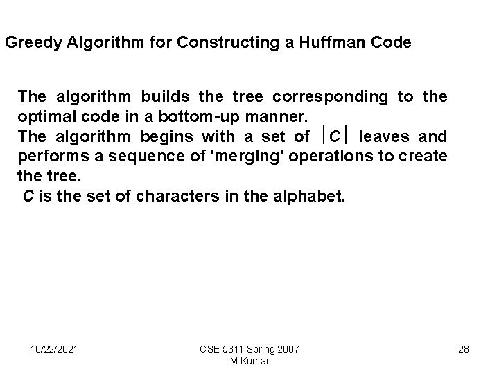
Greedy Algorithm for Constructing a Huffman Code The algorithm builds the tree corresponding to the optimal code in a bottom-up manner. The algorithm begins with a set of C leaves and performs a sequence of 'merging' operations to create the tree. C is the set of characters in the alphabet. 10/22/2021 CSE 5311 Spring 2007 M Kumar 28

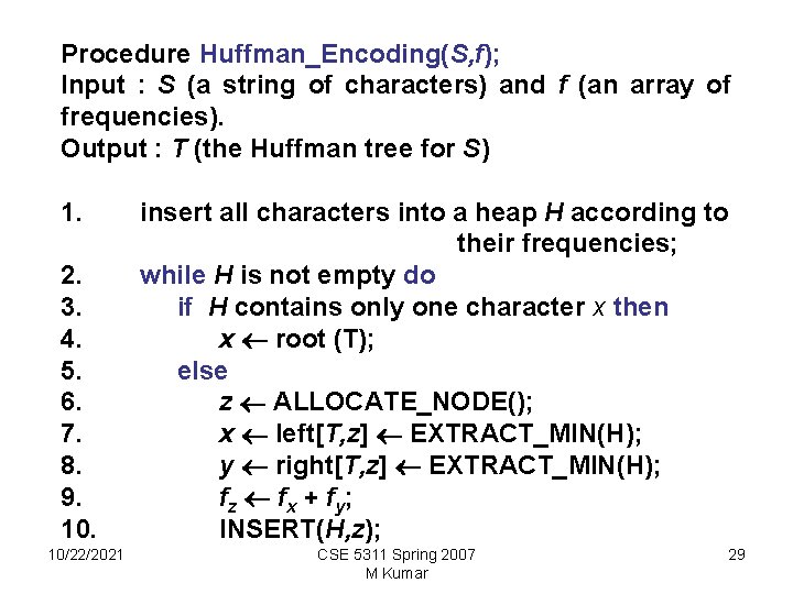
Procedure Huffman_Encoding(S, f); Input : S (a string of characters) and f (an array of frequencies). Output : T (the Huffman tree for S) 1. 2. 3. 4. 5. 6. 7. 8. 9. 10/22/2021 insert all characters into a heap H according to their frequencies; while H is not empty do if H contains only one character x then x root (T); else z ALLOCATE_NODE(); x left[T, z] EXTRACT_MIN(H); y right[T, z] EXTRACT_MIN(H); fz fx + fy ; INSERT(H, z); CSE 5311 Spring 2007 M Kumar 29

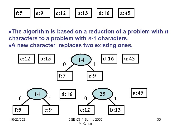
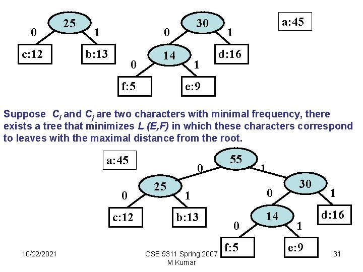
f: 5 e: 9 c: 12 b: 13 d: 16 a: 45 ·The algorithm is based on a reduction of a problem with n characters to a problem with n-1 characters. ·A new character replaces two existing ones. c: 12 b: 13 14 0 1 f: 5 0 f: 5 10/22/2021 14 1 e: 9 d: 16 a: 45 e: 9 d: 16 0 25 c: 12 CSE 5311 Spring 2007 M Kumar 1 a: 45 b: 13 30

0 c: 12 25 1 0 b: 13 14 0 f: 5 30 1 a: 45 1 d: 16 e: 9 Suppose Ci and Cj are two characters with minimal frequency, there exists a tree that minimizes L (E, F) in which these characters correspond to leaves with the maximal distance from the root. a: 45 0 c: 12 10/22/2021 0 25 55 1 1 0 b: 13 14 CSE 5311 Spring 2007 M Kumar 0 f: 5 30 1 e: 9 1 d: 16 31

0 100 1 a: 45 55 0 25 0 c: 12 1 0 b: 13 14 0 f: 5 0 101 10/22/2021 100 111 1 1101 30 1 d: 16 1 e: 9 1100 CSE 5311 Spring 2007 M Kumar 32

Complexity of the algorithm Building a heap in step 1 takes O(n) time Insertions (steps 7 and 8) and deletions (step 10) on H take O (log n) time each Therefore Steps 2 through 10 take O(n logn) time Thus the overall complexity of the algorithm is O( n logn ). 10/22/2021 CSE 5311 Spring 2007 M Kumar 33

• The fractional knapsack problem • Limited supply of each item • Each item has a size and a value per unit (e. g. , Pound) – greedy strategy • Compute value per Pound for each item • Arrange these in non-increasing order • Fill sack with the item of greatest value per pound until either the item is exhausted or the sack is full • If sack is not full, fill the remainder with the next item in the list • Repeat until sack is full How about a 0 -1 Knapsack? ? Can we use Greedy strategy? 10/22/2021 CSE 5311 Spring 2007 M Kumar 34