Introduction to Algorithms Greedy Algorithms and Graphs Graphs

Introduction to Algorithms: Greedy Algorithms (and Graphs)

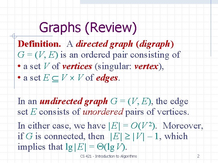
Graphs (Review) Definition. A directed graph (digraph) G = (V, E) is an ordered pair consisting of • a set V of vertices (singular: vertex), • a set E V V of edges. In an undirected graph G = (V, E), the edge set E consists of unordered pairs of vertices. In either case, we have | E | = O(V 2). Moreover, if G is connected, then | E | | V | – 1, which implies that lg | E | = (lg V). CS 421 - Introduction to Algorithms 2

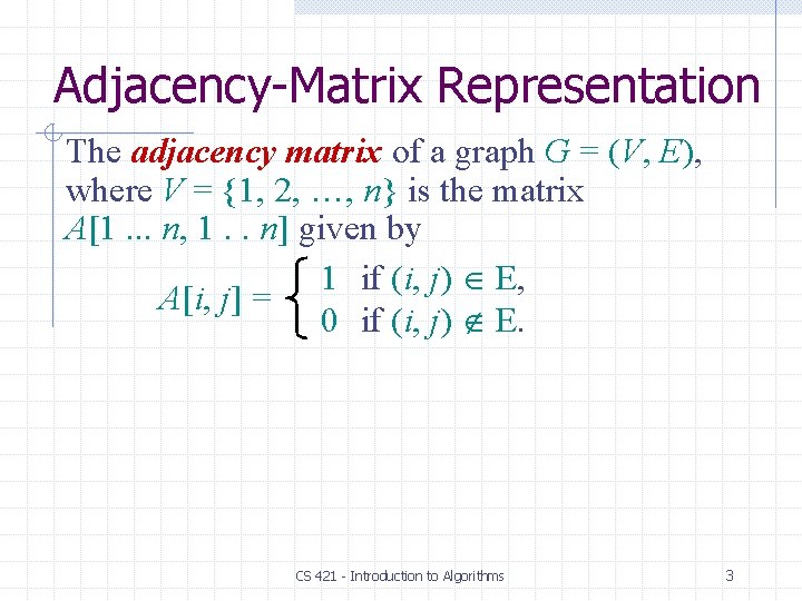
Adjacency-Matrix Representation The adjacency matrix of a graph G = (V, E), where V = {1, 2, …, n} is the matrix A[1. . . n, 1. . n] given by 1 if (i, j) E, A[i, j] = 0 if (i, j) E. CS 421 - Introduction to Algorithms 3

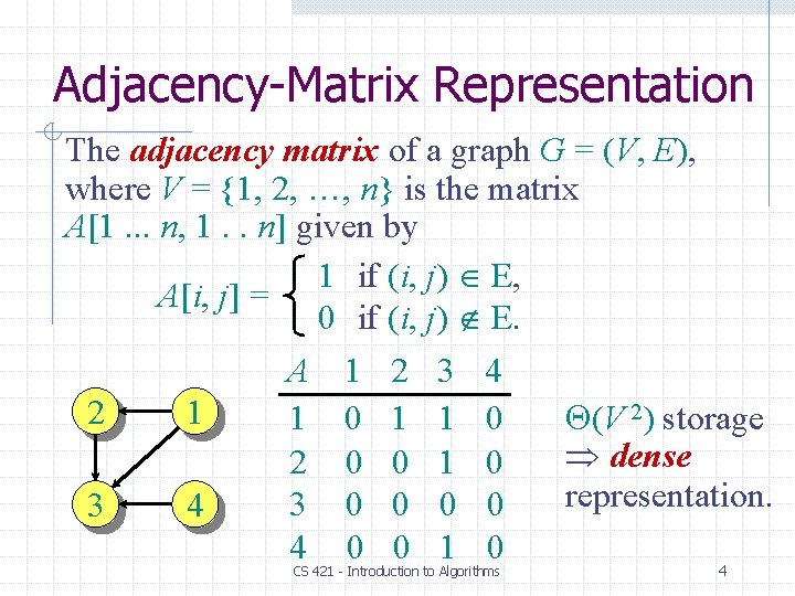
Adjacency-Matrix Representation The adjacency matrix of a graph G = (V, E), where V = {1, 2, …, n} is the matrix A[1. . . n, 1. . n] given by 1 if (i, j) E, A[i, j] = 0 if (i, j) E. A 1 2 3 4 2 1 (V 2) storage 1 0 1 1 0 dense 2 0 0 1 0 representation. 3 0 0 3 4 4 0 0 1 0 4 CS 421 - Introduction to Algorithms

Adjacency-List Representation An adjacency list of a vertex v V is the list Adj[v] of vertices adjacent to v. 2 1 3 4 Adj[1] = {2, 3} Adj[2] = {3} Adj[3] = {} Adj[4] = {3} CS 421 - Introduction to Algorithms 5

Adjacency-List Representation An adjacency list of a vertex v V is the list Adj[v] of vertices adjacent to v. 2 1 3 4 Adj[1] = {2, 3} Adj[2] = {3} Adj[3] = {} Adj[4] = {3} For undirected graphs, | Adj[v] | = degree(v). For digraphs, | Adj[v] | = out-degree(v). CS 421 - Introduction to Algorithms 6

Adjacency-List Representation An adjacency list of a vertex v V is the list Adj[v] of vertices adjacent to v. 2 1 3 4 Adj[1] = {2, 3} Adj[2] = {3} Adj[3] = {} Adj[4] = {3} For undirected graphs, | Adj[v] | = degree(v). For digraphs, | Adj[v] | = out-degree(v). Handshaking Lemma: v V = 2| E | for undirected graphs adjacency lists use (V + E) storage — a sparse representation (for either type of graph). 7

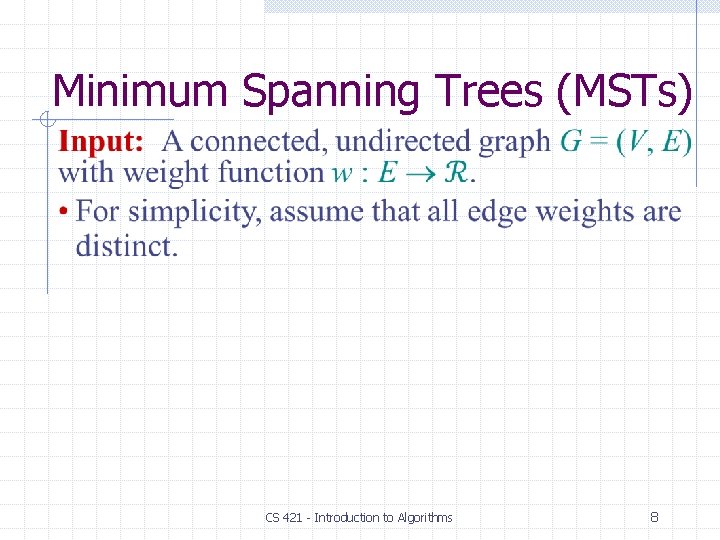
Minimum Spanning Trees (MSTs) CS 421 - Introduction to Algorithms 8

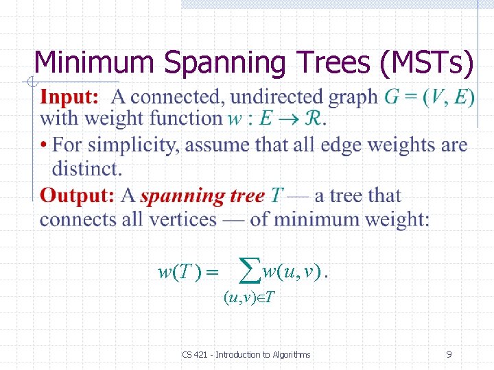
Minimum Spanning Trees (MSTs) w(T ) w(u, v). (u, v) T CS 421 - Introduction to Algorithms 9

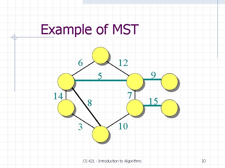
Example of MST 6 12 9 5 14 8 3 7 15 10 CS 421 - Introduction to Algorithms 10

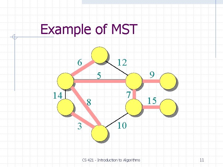
Example of MST 6 12 9 5 14 8 3 7 15 10 CS 421 - Introduction to Algorithms 11

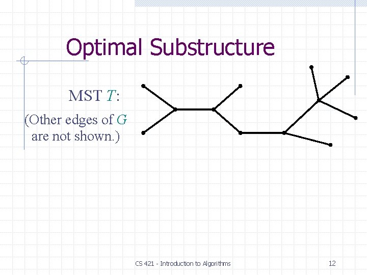
Optimal Substructure MST T: (Other edges of G are not shown. ) CS 421 - Introduction to Algorithms 12

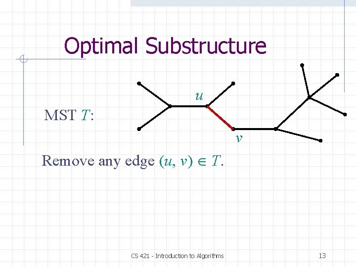
Optimal Substructure u MST T: v Remove any edge (u, v) T. CS 421 - Introduction to Algorithms 13

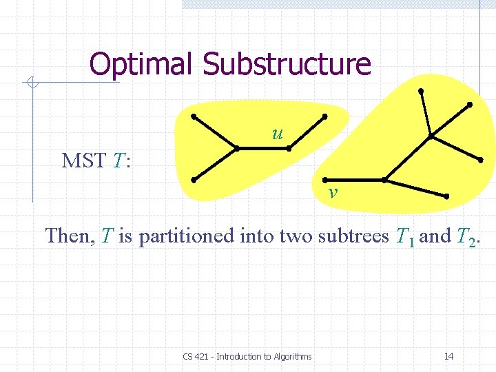
Optimal Substructure u MST T: v Then, T is partitioned into two subtrees T 1 and T 2. CS 421 - Introduction to Algorithms 14

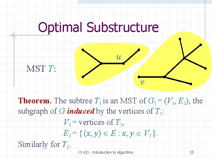
Optimal Substructure u MST T: v Theorem. The subtree T 1 is an MST of G 1 = (V 1, E 1), the subgraph of G induced by the vertices of T 1: V 1 = vertices of T 1, E 1 = { (x, y) E : x, y V 1 }. Similarly for T 2. CS 421 - Introduction to Algorithms 15

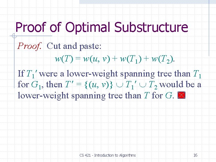
Proof of Optimal Substructure Proof. Cut and paste: w(T) = w(u, v) + w(T 1) + w(T 2). If T 1 were a lower-weight spanning tree than T 1 for G 1, then T = {(u, v)} T 1 T 2 would be a lower-weight spanning tree than T for G. CS 421 - Introduction to Algorithms 16

Proof of Optimal Substructure Proof. Cut and paste: w(T) = w(u, v) + w(T 1) + w(T 2). Do we also have overlapping sub-problems? • Yes. Great, then dynamic programming may work! • Yes, but MST exhibits another powerful property which leads to an even more efficient algorithm. CS 421 - Introduction to Algorithms 17

Hallmark for “Greedy” Algorithms Greedy-choice property A locally optimal choice is globally optimal. CS 421 - Introduction to Algorithms 18

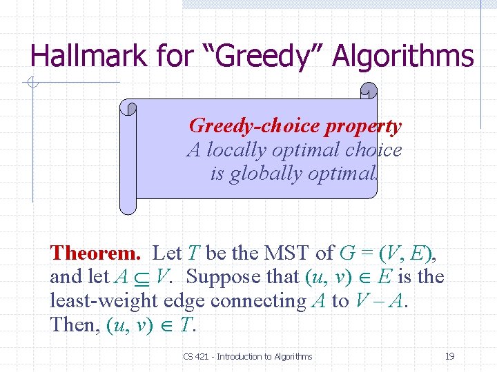
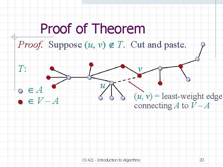
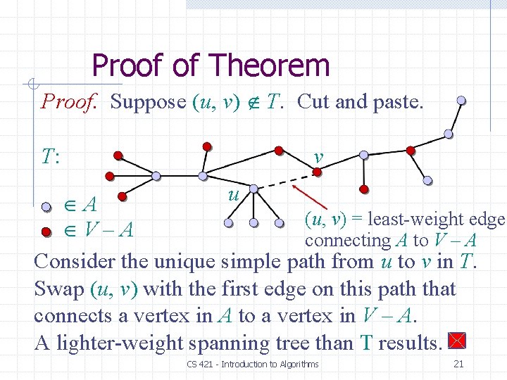
Hallmark for “Greedy” Algorithms Greedy-choice property A locally optimal choice is globally optimal. Theorem. Let T be the MST of G = (V, E), and let A V. Suppose that (u, v) E is the least-weight edge connecting A to V – A. Then, (u, v) T. CS 421 - Introduction to Algorithms 19

Proof of Theorem Proof. Suppose (u, v) T. Cut and paste. T: v A V–A u (u, v) = least-weight edge connecting A to V – A CS 421 - Introduction to Algorithms 20

Proof of Theorem Proof. Suppose (u, v) T. Cut and paste. T: v u A (u, v) = least-weight edge V–A connecting A to V – A Consider the unique simple path from u to v in T. Swap (u, v) with the first edge on this path that connects a vertex in A to a vertex in V – A. A lighter-weight spanning tree than T results. CS 421 - Introduction to Algorithms 21

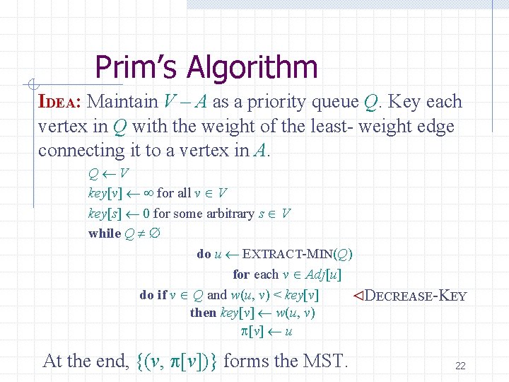
Prim’s Algorithm IDEA: Maintain V – A as a priority queue Q. Key each vertex in Q with the weight of the least- weight edge connecting it to a vertex in A. Q V key[v] for all v V key[s] 0 for some arbitrary s V while Q do u EXTRACT-MIN(Q) for each v Adj[u] do if v Q and w(u, v) < key[v] ⊳DECREASE-KEY then key[v] w(u, v) [v] u At the end, {(v, [v])} forms the MST. 22

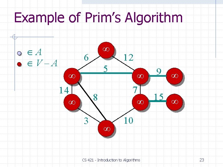
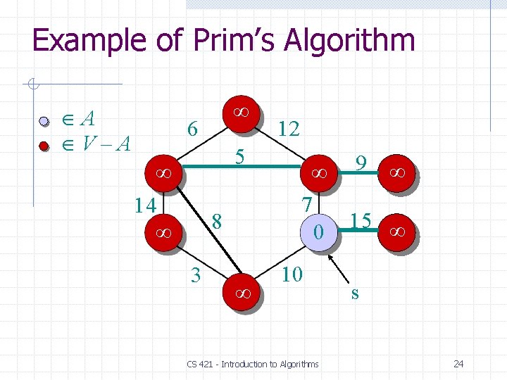
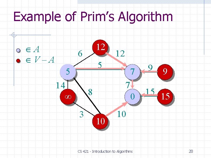
Example of Prim’s Algorithm A V–A 6 5 14 8 3 12 9 7 15 10 CS 421 - Introduction to Algorithms 23

Example of Prim’s Algorithm A V–A 6 5 14 8 3 12 9 7 15 0 10 CS 421 - Introduction to Algorithms s 24

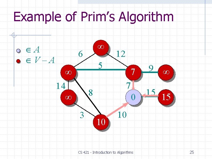
Example of Prim’s Algorithm A V–A 6 5 14 8 3 10 12 7 7 0 9 15 15 10 CS 421 - Introduction to Algorithms 25

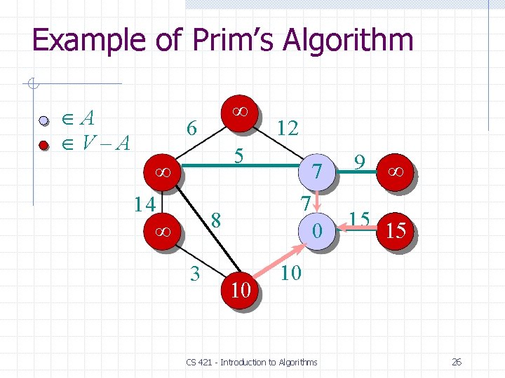
Example of Prim’s Algorithm A V–A 6 12 5 14 9 0 15 15 7 8 3 7 10 CS 421 - Introduction to Algorithms 26

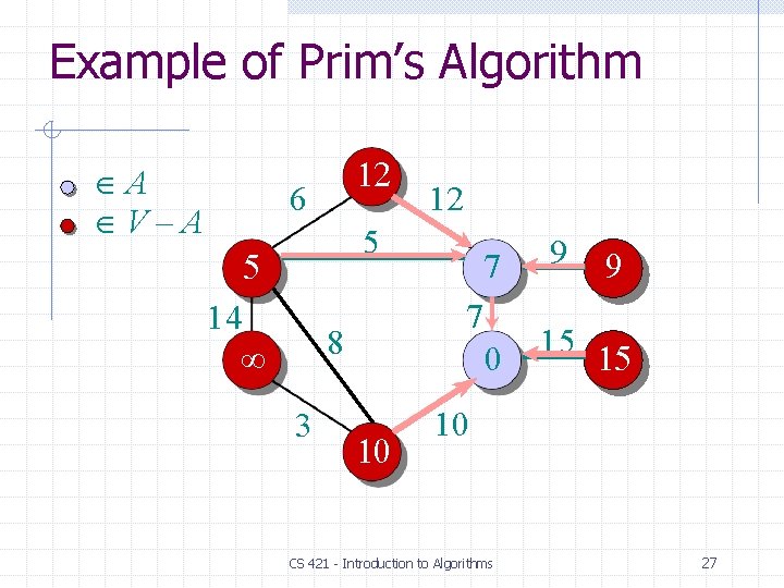
Example of Prim’s Algorithm A V–A 12 6 12 5 5 14 9 0 15 15 7 8 3 7 10 9 10 CS 421 - Introduction to Algorithms 27

Example of Prim’s Algorithm A V–A 12 6 12 5 5 14 9 0 15 15 7 8 3 7 10 9 10 CS 421 - Introduction to Algorithms 28

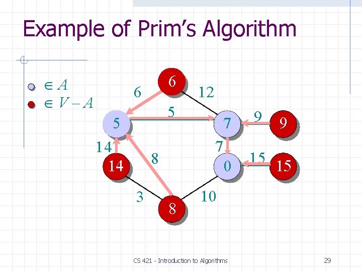
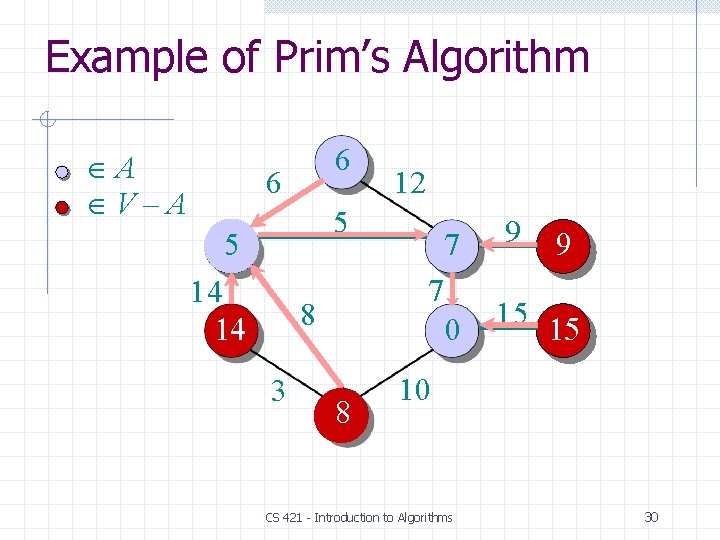
Example of Prim’s Algorithm A V–A 6 6 12 5 5 14 14 9 0 15 15 7 8 3 7 8 9 10 CS 421 - Introduction to Algorithms 29

Example of Prim’s Algorithm A V–A 6 6 12 5 5 14 14 9 0 15 15 7 8 3 7 8 9 10 CS 421 - Introduction to Algorithms 30

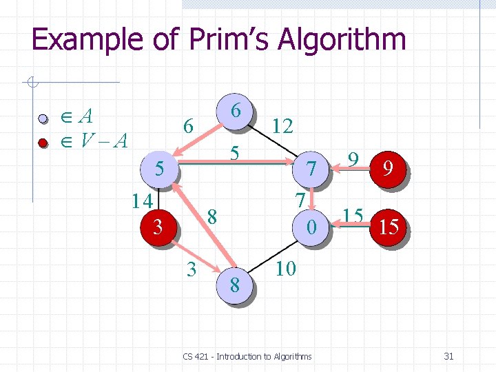
Example of Prim’s Algorithm A V–A 6 6 12 5 5 14 3 9 0 15 15 7 8 3 7 8 9 10 CS 421 - Introduction to Algorithms 31

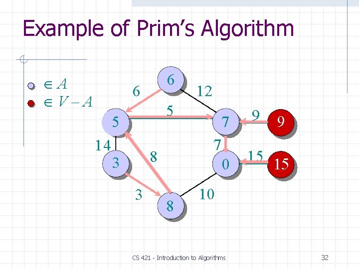
Example of Prim’s Algorithm A V–A 6 6 5 5 14 12 3 9 0 15 15 7 8 3 7 8 9 10 CS 421 - Introduction to Algorithms 32

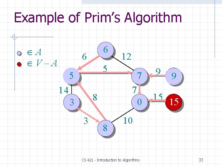
Example of Prim’s Algorithm A V–A 6 6 12 5 5 14 3 9 0 15 15 7 8 3 7 8 9 10 CS 421 - Introduction to Algorithms 33

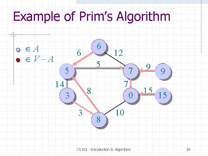
Example of Prim’s Algorithm A V–A 6 6 12 5 5 14 7 8 3 3 7 0 8 9 15 10 CS 421 - Introduction to Algorithms 34

Analysis of Prim‘s Algorithm Q V key[v] for all v V key[s] 0 for some arbitrary s V while Q do u EXTRACT-MIN(Q) for each v Adj[u] do if v Q and w(u, v) < key[v] then key[v] w(u, v) [v] u CS 421 - Introduction to Algorithms 35

Analysis of Prim‘s Algorithm Q V (V) key[v] for all v V total key[s] 0 for some arbitrary s V while Q do u EXTRACT-MIN(Q) for each v Adj[u] |V | do if v Q and w(u, v) < key[v] times degree(u) times then key[v] w(u, v) [v] u Handshaking Lemma (E) implicit DECREASE-KEY’s. CS 421 - Introduction to Algorithms 36

Analysis of Prim‘s Algorithm Q V (V) key[v] for all v V total key[s] 0 for some arbitrary s V while Q do u EXTRACT-MIN(Q) for each v Adj[u] |V | do if v Q and w(u, v) < key[v] times degree(u) times then key[v] w(u, v) [v] u Time = (V)·TEXTRACT-MIN + (E)·TDECREASE-KEY CS 421 - Introduction to Algorithms 37

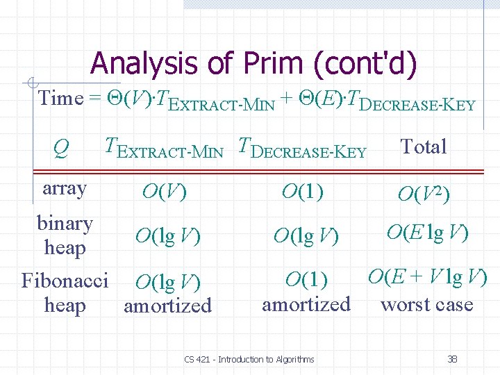
Analysis of Prim (cont'd) Time = (V)·TEXTRACT-MIN + (E)·TDECREASE-KEY Q TEXTRACT-MIN TDECREASE-KEY Total array O(V) O(1) O(V 2) binary heap O(lg V) O(E lg V) Fibonacci O(lg V) heap amortized O(E + V lg V) O(1) amortized worst case CS 421 - Introduction to Algorithms 38

MST Algorithms • Kruskal’s algorithm (see CLRS): • Uses the disjoint-set data structure • Running time = O(E lg V). • Best to date: • • • Karger, Klein, and Tarjan [1993]. Randomized algorithm. O(V + E) expected time. CS 421 - Introduction to Algorithms 39