Algorithm Techniques Techniques Divide and Conquer Dynamic Programming

Algorithm Techniques

Techniques • Divide and Conquer • Dynamic Programming • Greedy Algorithm

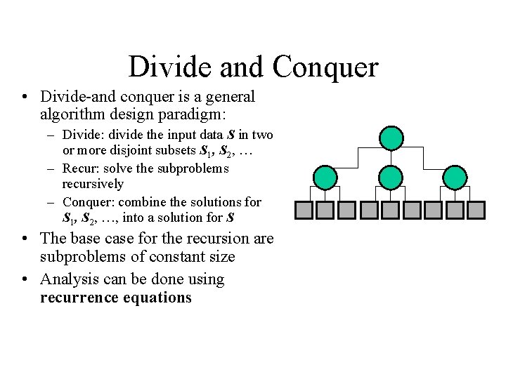
Divide and Conquer • Divide-and conquer is a general algorithm design paradigm: – Divide: divide the input data S in two or more disjoint subsets S 1, S 2, … – Recur: solve the subproblems recursively – Conquer: combine the solutions for S 1, S 2, …, into a solution for S • The base case for the recursion are subproblems of constant size • Analysis can be done using recurrence equations

Divide and Conquer • Merge Sort • Quick Sort • Closet Point

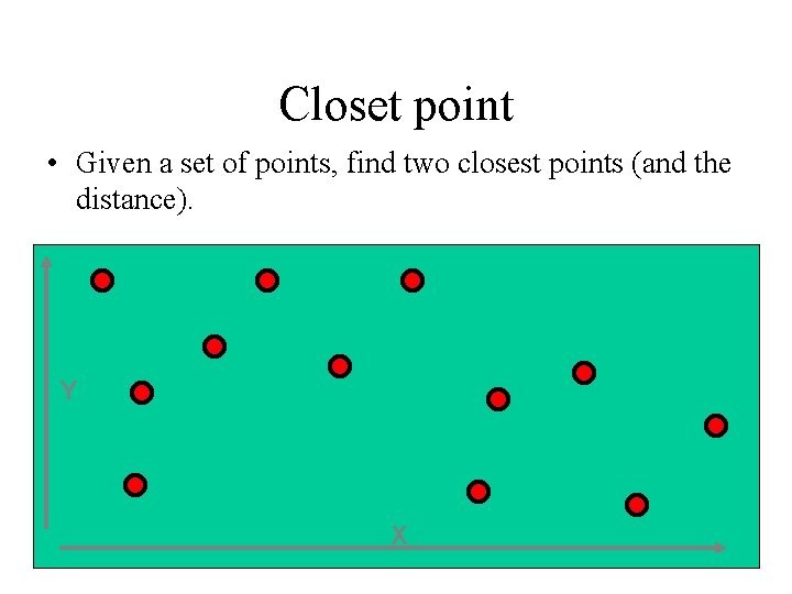
Closet point • Given a set of points, find two closest points (and the distance). Y X

Closet point • Brute Force – Try all possibilities. – Guarantees correct answer – Easy to program • Point #1 has n – 1 distance computations and compares • Point #2 has n – 2 distance computations and compares • … O(n 2)

Closet point • DIVIDE: partition the data set into smaller subsets • CONQUER: solve for closest points in each subset COMBINE: closest point is either d. L, d. M, or d. R d. M – closet pair of points w/ one point in each set

Closet point (Solving d. M ) • d = minimum (d. L , d. R) • Only need to consider points within d of L For any points in corridor, compute distances within some window

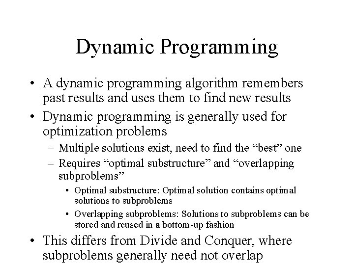
Dynamic Programming • A dynamic programming algorithm remembers past results and uses them to find new results • Dynamic programming is generally used for optimization problems – Multiple solutions exist, need to find the “best” one – Requires “optimal substructure” and “overlapping subproblems” • Optimal substructure: Optimal solution contains optimal solutions to subproblems • Overlapping subproblems: Solutions to subproblems can be stored and reused in a bottom-up fashion • This differs from Divide and Conquer, where subproblems generally need not overlap

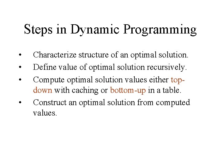
Steps in Dynamic Programming • • Characterize structure of an optimal solution. Define value of optimal solution recursively. Compute optimal solution values either topdown with caching or bottom-up in a table. Construct an optimal solution from computed values.

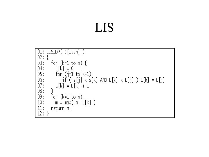
LIS

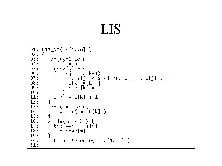
LIS

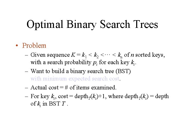
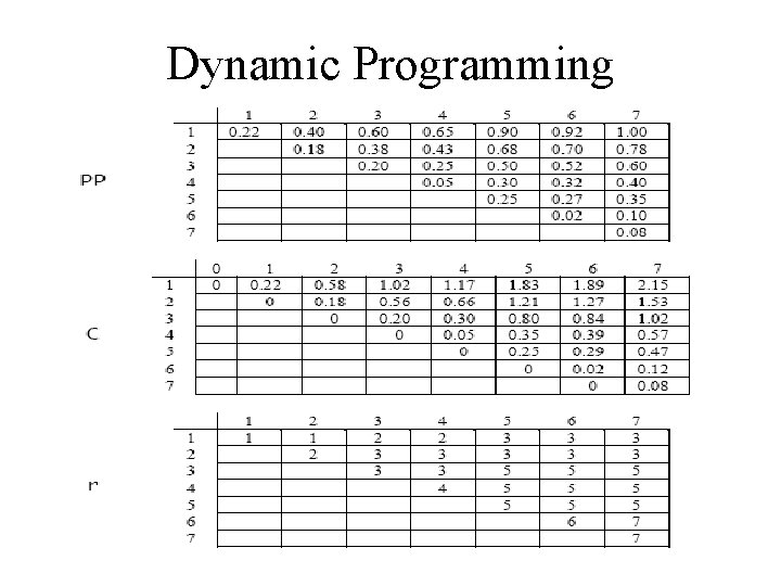
Optimal Binary Search Trees • Problem – Given sequence K = k 1 < k 2 <··· < kn of n sorted keys, with a search probability pi for each key ki. – Want to build a binary search tree (BST) with minimum expected search cost. – Actual cost = # of items examined. – For key ki, cost = depth. T(ki)+1, where depth. T(ki) = depth of ki in BST T.

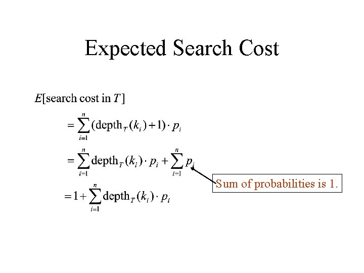
Expected Search Cost Sum of probabilities is 1.

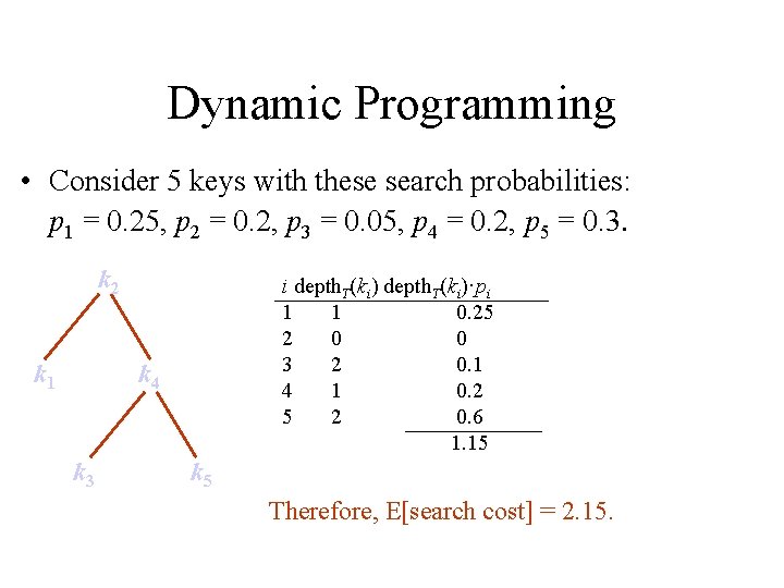
Dynamic Programming • Consider 5 keys with these search probabilities: p 1 = 0. 25, p 2 = 0. 2, p 3 = 0. 05, p 4 = 0. 2, p 5 = 0. 3. k 2 k 1 i depth. T(ki)·pi 1 1 0. 25 2 0 0 3 2 0. 1 4 1 0. 2 5 2 0. 6 1. 15 k 4 k 3 k 5 Therefore, E[search cost] = 2. 15.

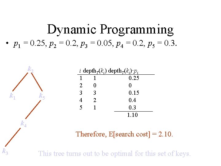
Dynamic Programming • p 1 = 0. 25, p 2 = 0. 2, p 3 = 0. 05, p 4 = 0. 2, p 5 = 0. 3. k 2 k 1 k 5 i depth. T(ki)·pi 1 1 0. 25 2 0 0 3 3 0. 15 4 2 0. 4 5 1 0. 3 1. 10 k 4 Therefore, E[search cost] = 2. 10. k 3 This tree turns out to be optimal for this set of keys.

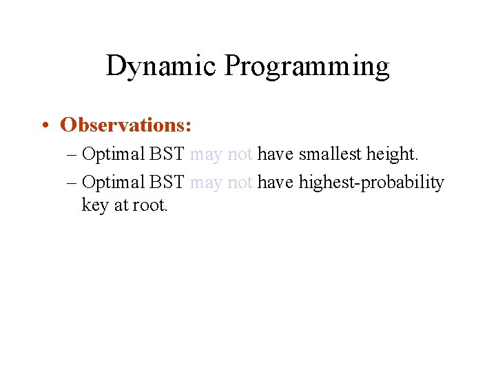
Dynamic Programming • Observations: – Optimal BST may not have smallest height. – Optimal BST may not have highest-probability key at root.

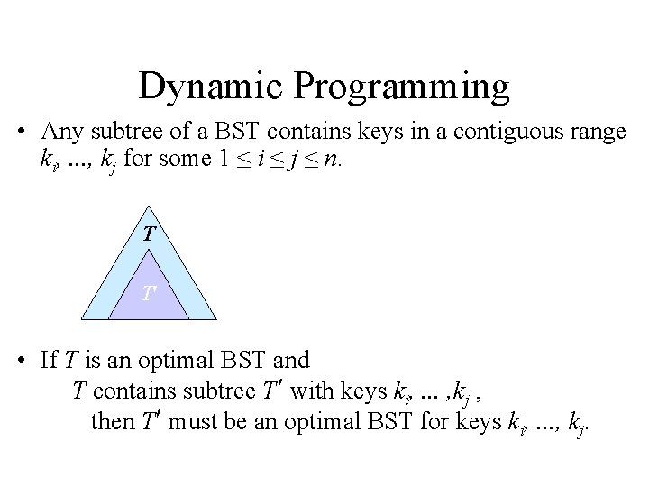
Dynamic Programming • Any subtree of a BST contains keys in a contiguous range ki, . . . , kj for some 1 ≤ i ≤ j ≤ n. T T • If T is an optimal BST and T contains subtree T with keys ki, . . . , kj , then T must be an optimal BST for keys ki, . . . , kj.

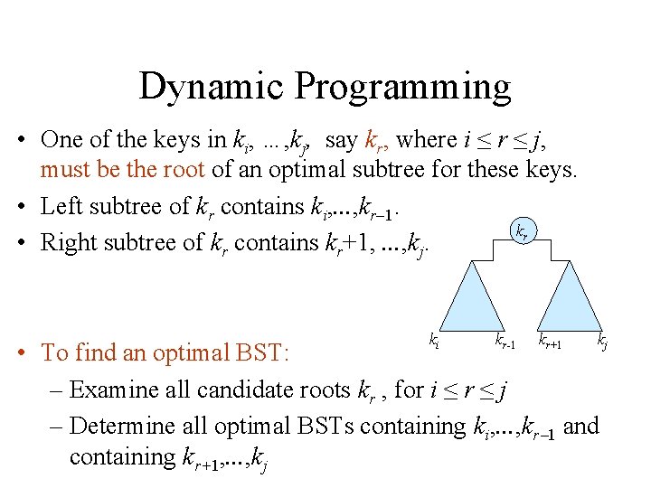
Dynamic Programming • One of the keys in ki, …, kj, say kr, where i ≤ r ≤ j, must be the root of an optimal subtree for these keys. • Left subtree of kr contains ki, . . . , kr 1. kr • Right subtree of kr contains kr+1, . . . , kj. ki kr-1 kr+1 kj • To find an optimal BST: – Examine all candidate roots kr , for i ≤ r ≤ j – Determine all optimal BSTs containing ki, . . . , kr 1 and containing kr+1, . . . , kj

Dynamic Programming • One of the keys in ki, …, kj, say kr, where i ≤ r ≤ j, must be the root of an optimal subtree for these keys. • Left subtree of kr contains ki, . . . , kr 1. kr • Right subtree of kr contains kr+1, . . . , kj. ki kr-1 kr+1 kj • To find an optimal BST: – Examine all candidate roots kr , for i ≤ r ≤ j – Determine all optimal BSTs containing ki, . . . , kr 1 and containing kr+1, . . . , kj

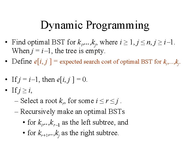
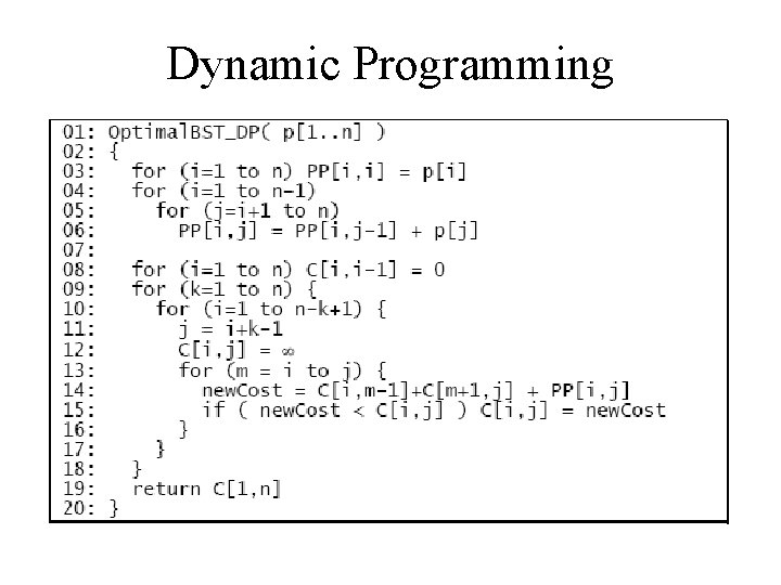
Dynamic Programming • Find optimal BST for ki, . . . , kj, where i ≥ 1, j ≤ n, j ≥ i 1. When j = i 1, the tree is empty. • Define e[i, j ] = expected search cost of optimal BST for ki, . . . , kj. • If j = i 1, then e[i, j ] = 0. • If j ≥ i, – Select a root kr, for some i ≤ r ≤ j. – Recursively make an optimal BSTs • for ki, . . , kr 1 as the left subtree, and • for kr+1, . . , kj as the right subtree.

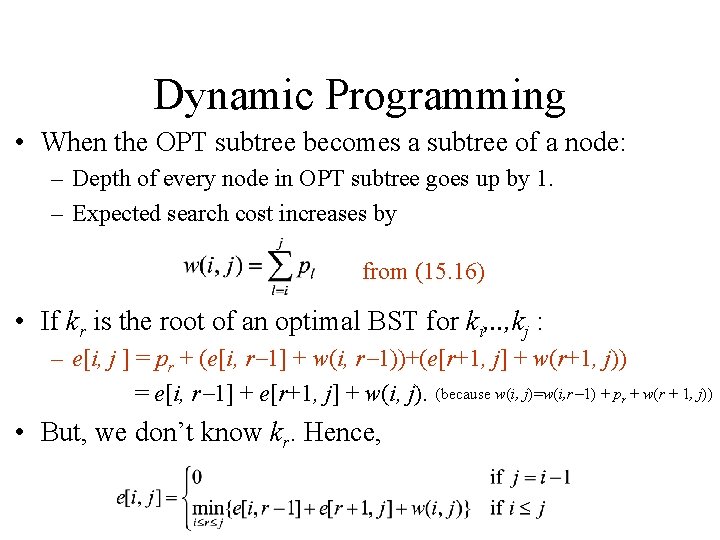
Dynamic Programming • When the OPT subtree becomes a subtree of a node: – Depth of every node in OPT subtree goes up by 1. – Expected search cost increases by from (15. 16) • If kr is the root of an optimal BST for ki, . . , kj : – e[i, j ] = pr + (e[i, r 1] + w(i, r 1))+(e[r+1, j] + w(r+1, j)) = e[i, r 1] + e[r+1, j] + w(i, j). (because w(i, j)=w(i, r 1) + pr + w(r + 1, j)) • But, we don’t know kr. Hence,

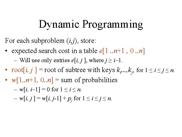
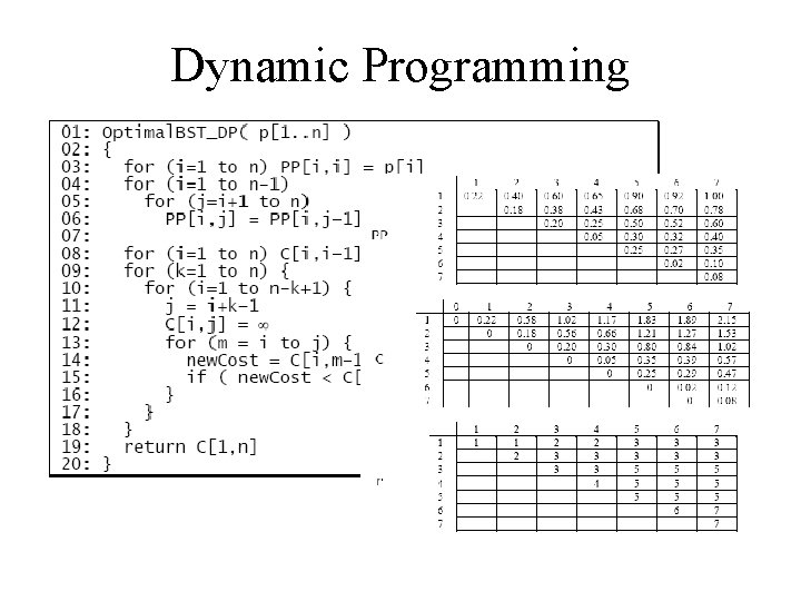
Dynamic Programming For each subproblem (i, j), store: • expected search cost in a table e[1. . n+1 , 0. . n] – Will use only entries e[i, j ], where j ≥ i 1. • root[i, j ] = root of subtree with keys ki, . . , kj, for 1 ≤ i ≤ j ≤ n. • w[1. . n+1, 0. . n] = sum of probabilities – w[i, i 1] = 0 for 1 ≤ i ≤ n. – w[i, j ] = w[i, j-1] + pj for 1 ≤ i ≤ j ≤ n.

Dynamic Programming

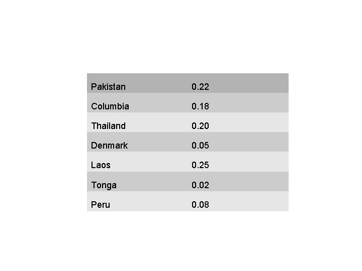
Pakistan 0. 22 Columbia 0. 18 Thailand 0. 20 Denmark 0. 05 Laos 0. 25 Tonga 0. 02 Peru 0. 08

Dynamic Programming

Dynamic Programming

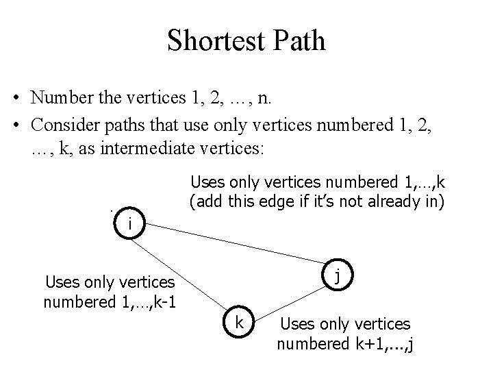
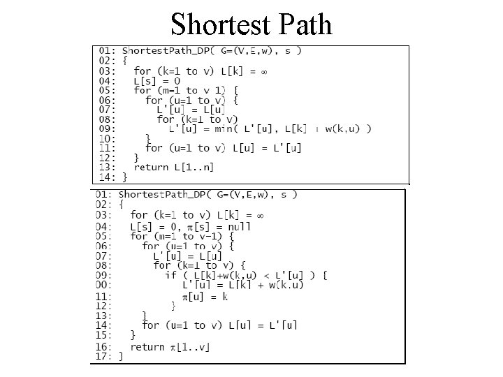
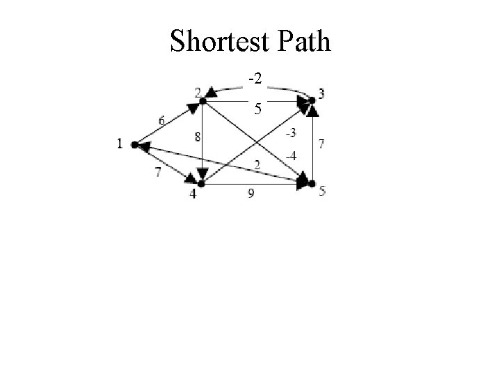
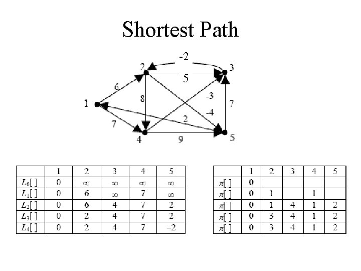
Shortest Path • Number the vertices 1, 2, …, n. • Consider paths that use only vertices numbered 1, 2, …, k, as intermediate vertices: Uses only vertices numbered 1, …, k (add this edge if it’s not already in) i j Uses only vertices numbered 1, …, k-1 k Uses only vertices numbered k+1, . . . , j

Shortest Path

Shortest Path -2 5

Shortest Path -2 5

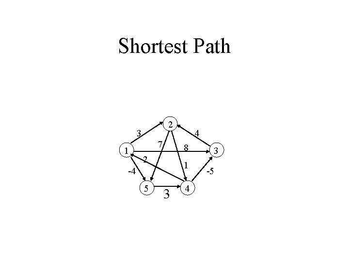
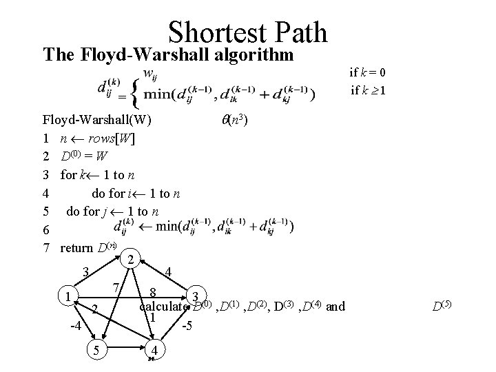
Shortest Path 2 3 1 7 8 2 1 -4 5 4 3 -5

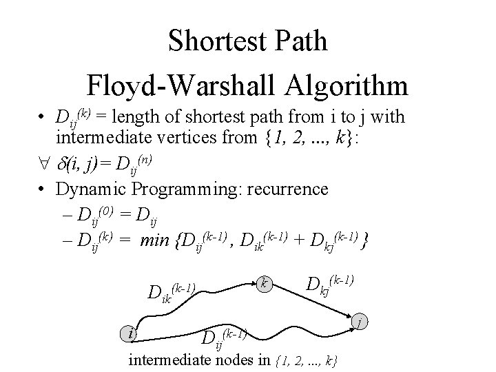
Shortest Path Floyd-Warshall Algorithm • Dij(k) = length of shortest path from i to j with intermediate vertices from {1, 2, . . . , k}: (i, j)= Dij(n) • Dynamic Programming: recurrence – Dij(0) = Dij – Dij(k) = min {Dij(k-1) , Dik(k-1) + Dkj(k-1) } Dik i k (k-1) Dij(k-1) Dkj(k-1) intermediate nodes in {1, 2, . . . , k} j

Shortest Path The Floyd-Warshall algorithm = if k = 0 if k 1 { Floyd-Warshall(W) (n 3) 1 n rows[W] 2 D(0) = W 3 for k 1 to n 4 do for i 1 to n 5 do for j 1 to n 6 7 return D(n) 2 3 4 7 8 1 3 (0) (1) (2) (3) (4) calculate D , D , D and 2 1 -4 -5 5 4 36 D(5)

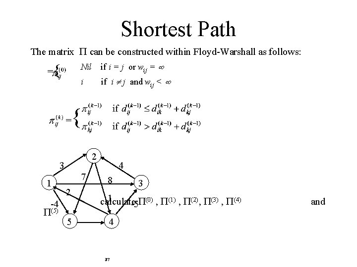
Shortest Path The matrix can be constructed within Floyd-Warshall as follows: = { = Nil if i = j or wij = i if i j and wij < { 2 3 1 -4 (5) 7 2 5 4 8 3 1 (0) (1) (2) (3) (4) calculate -5 , , 4 37 and

Greedy Algorithm • An optimization problem is one in which you want to find, not just a solution, but the best solution • A “greedy algorithm” sometimes works well for optimization problems • A greedy algorithm works in phases: At each phase: – You take the best you can get right now, without regard for future consequences – You hope that by choosing a local optimum at each step, you will end up at a global optimum

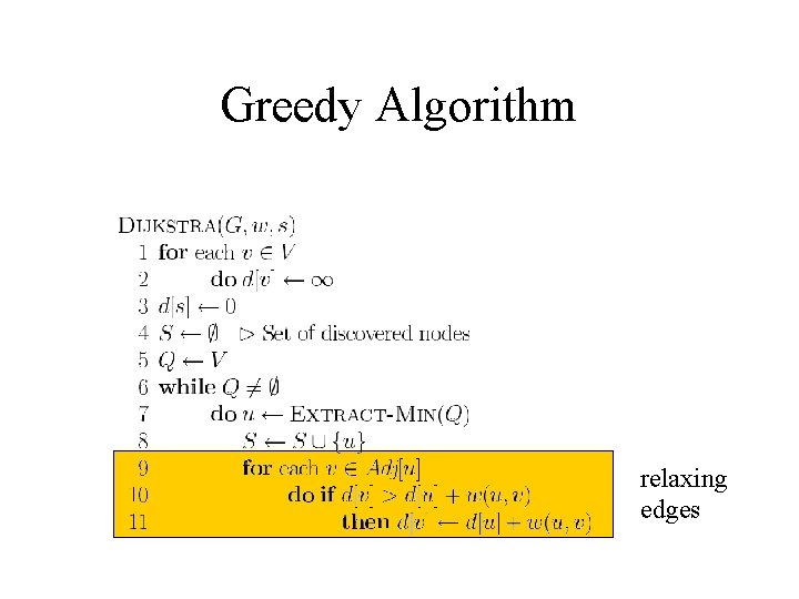
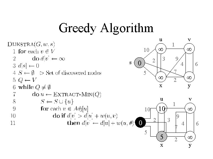
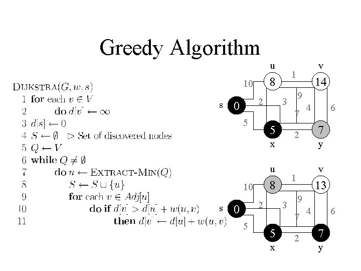
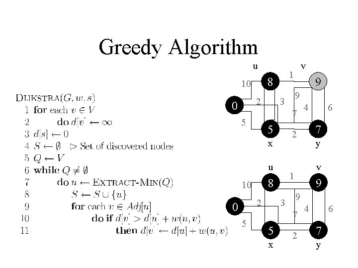
Dijkstra's Algorithm • Non-negative edge weights • Greedy, similar to Prim's algorithm for MST • Like breadth-first search (if all weights = 1, one can simply use BFS) • Use Q, a priority queue with keys v. dist (BFS used FIFO queue, here we use a PQ, which is reorganized whenever some dist decreases) • Basic idea – maintain a set S of solved vertices – at each step select "closest" vertex u, add it to S, and relax all edges from u

Greedy Algorithm relaxing edges

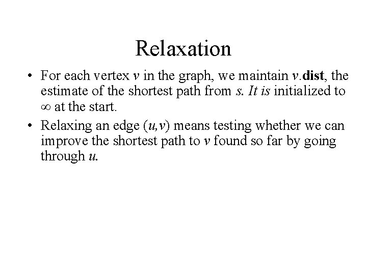
Relaxation • For each vertex v in the graph, we maintain v. dist, the estimate of the shortest path from s. It is initialized to at the start. • Relaxing an edge (u, v) means testing whether we can improve the shortest path to v found so far by going through u.

Greedy Algorithm u s 2 1 10 5 u s 5 3 y v 9 7 x 6 1 4 7 2 x 2 9 3 10 v 2 4 6 y

Greedy Algorithm u s 2 1 10 2 3 x y v 9 7 6 1 10 4 2 u 5 9 3 x 7 5 s v 2 4 6 y

Greedy Algorithm u 2 1 10 9 3 u 2 3 x y v 9 7 6 1 10 4 2 x 5 7 5 v 2 4 6 y

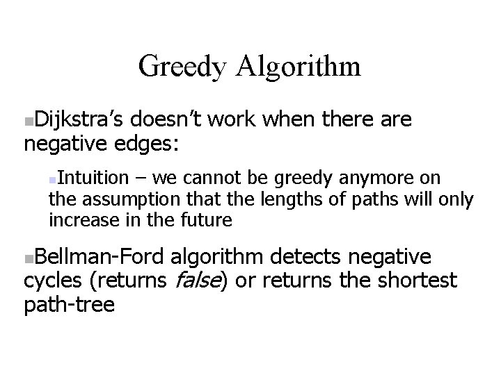
Greedy Algorithm Dijkstra’s doesn’t work when there are negative edges: Intuition – we cannot be greedy anymore on the assumption that the lengths of paths will only increase in the future Bellman-Ford algorithm detects negative cycles (returns false) or returns the shortest path-tree

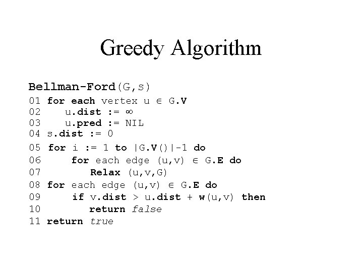
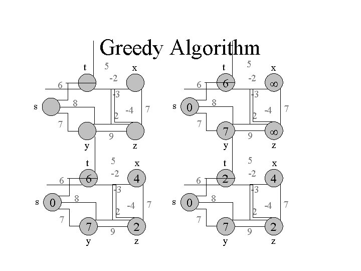
Greedy Algorithm Bellman-Ford(G, s) 01 02 03 04 05 06 07 08 09 10 11 for each vertex u G. V u. dist : = u. pred : = NIL s. dist : = 0 for i : = 1 to |G. V()|-1 do for each edge (u, v) G. E do Relax (u, v, G) for each edge (u, v) G. E do if v. dist > u. dist + w(u, v) then return false return true

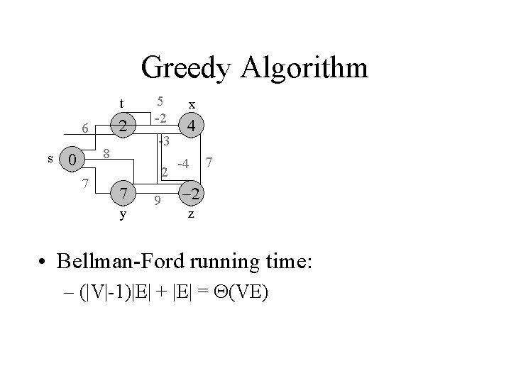
Greedy Algorithm t 6 2 7 y t 6 s 8 7 t x 9 5 -2 -3 2 y 9 6 -3 8 s 5 -2 7 -4 s 8 z y x t -4 z 6 7 s 8 7 -3 2 7 5 -2 9 5 -2 -3 2 y 9 x -4 7 z x -4 z 7

Greedy Algorithm t 6 s 8 7 5 -2 -3 2 y 9 x -4 7 z • Bellman-Ford running time: – (|V|-1)|E| + |E| = (VE)

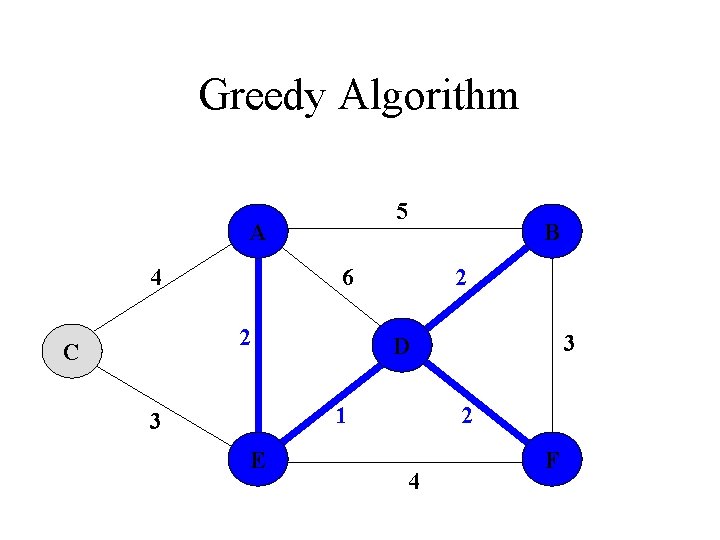
Greedy Algorithm Minimum- Spanning Trees Concrete example: computer connection 2. Definition of a Minimum- Spanning Tree 3. The Crucial Fact about Minimum- Spanning Trees 4. Algorithms to find Minimum- Spanning Trees - Kruskal‘s Algorithm - Prim‘s Algorithm

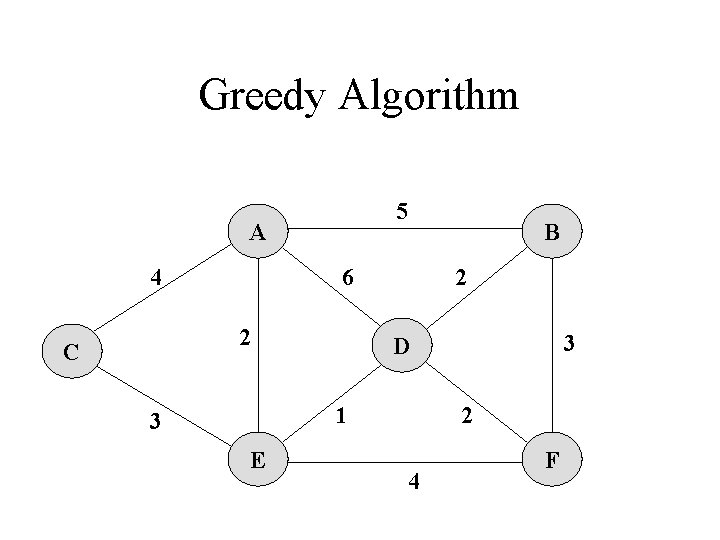
Greedy Algorithm Imagine: You wish to connect all the computers in an office building using the least amount of cable a weighted graph problem !! - Each vertex in a graph G represents a computer - Each edge represents the amount of cable needed to connect all computers

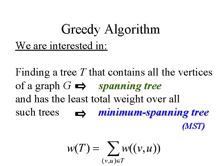
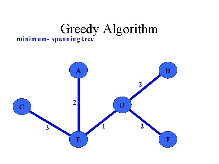
Greedy Algorithm We are interested in: Finding a tree T that contains all the vertices of a graph G spanning tree and has the least total weight over all such trees minimum-spanning tree (MST)

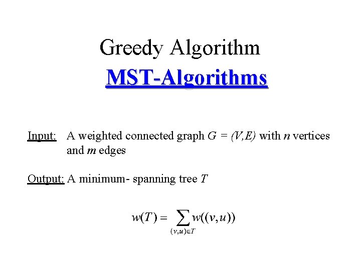
Greedy Algorithm MST-Algorithms Input: A weighted connected graph G = (V, E) with n vertices and m edges Output: A minimum- spanning tree T

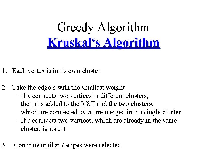
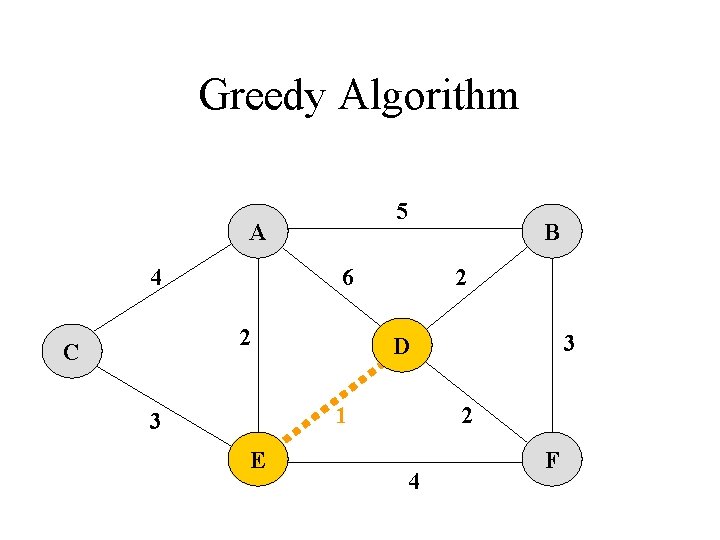
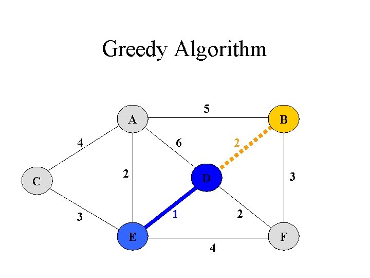
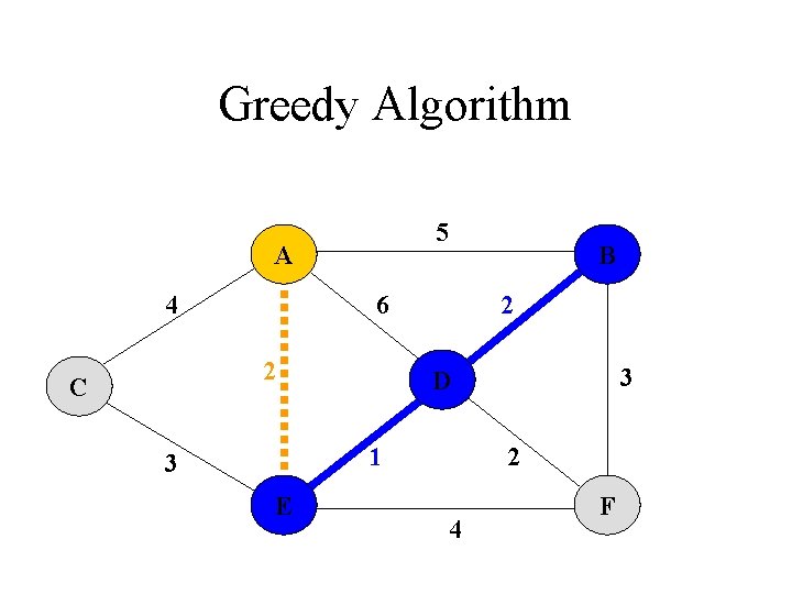
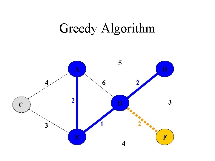
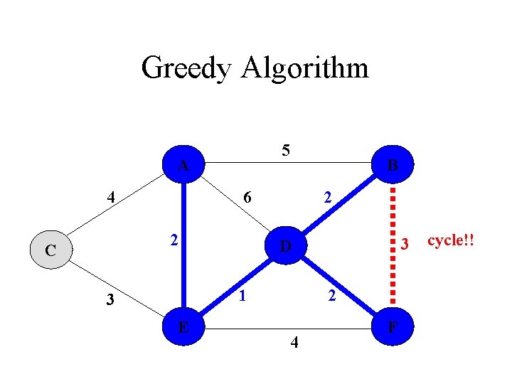
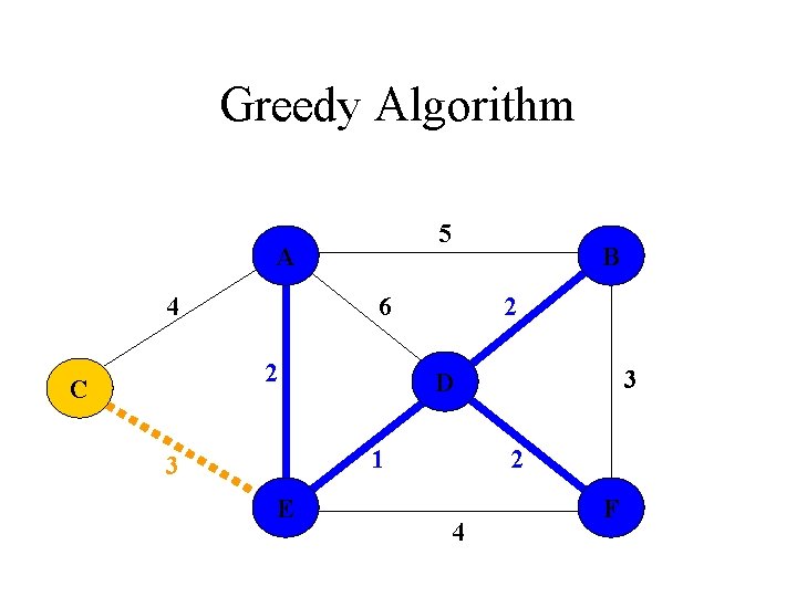
Greedy Algorithm Kruskal‘s Algorithm 1. Each vertex is in its own cluster 2. Take the edge e with the smallest weight - if e connects two vertices in different clusters, then e is added to the MST and the two clusters, which are connected by e, are merged into a single cluster - if e connects two vertices, which are already in the same cluster, ignore it 3. Continue until n-1 edges were selected

Greedy Algorithm 5 A 4 6 2 C B 2 1 3 E 3 D 2 4 F

Greedy Algorithm 5 A 4 6 2 C B 2 1 3 E 3 D 2 4 F

Greedy Algorithm 5 A 4 6 2 C B 2 1 3 E 3 D 2 4 F

Greedy Algorithm 5 A 4 6 2 C B 2 1 3 E 3 D 2 4 F

Greedy Algorithm 5 A 4 6 2 C B 2 1 3 E 3 D 2 4 F

Greedy Algorithm 5 A 4 6 2 C B 2 1 3 E 3 D 2 4 F cycle!!

Greedy Algorithm 5 A 4 6 2 C B 2 1 3 E 3 D 2 4 F

Greedy Algorithm 5 A 4 6 2 C B 2 1 3 E 3 D 2 4 F

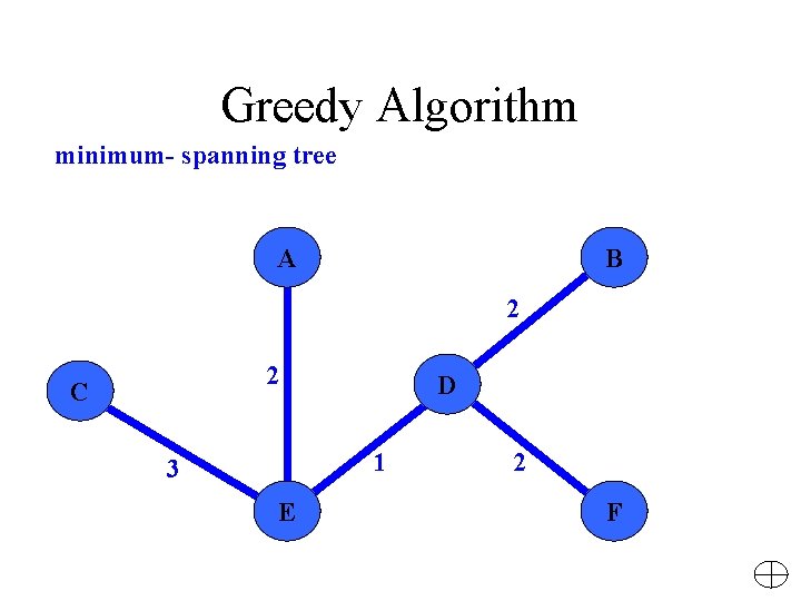
Greedy Algorithm minimum- spanning tree A B 2 2 C D 1 3 E 2 F

Greedy Algorithm Crucial Fact about MSTs Running time: O ( m log n ) By implementing queue Q as a heap, Q could be initialized in O ( m ) time and a vertex could be extracted in each iteration in O ( log n ) time

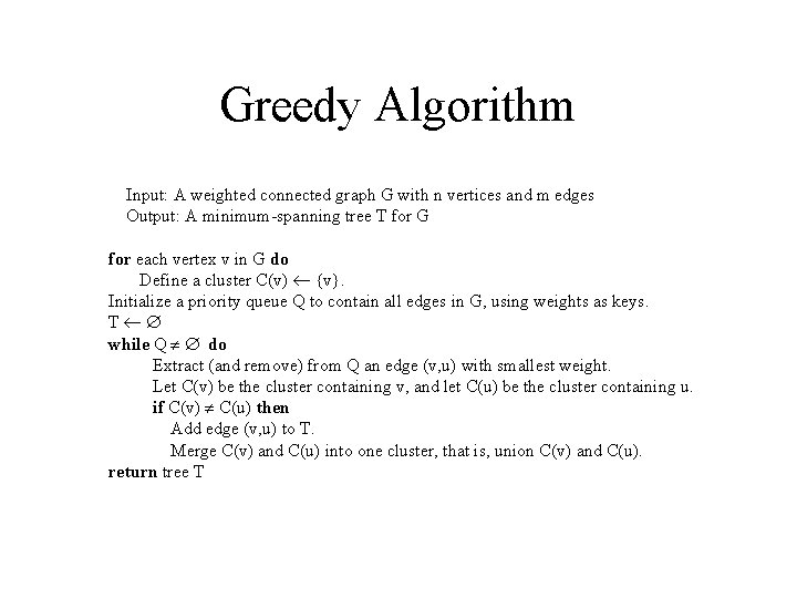
Greedy Algorithm Input: A weighted connected graph G with n vertices and m edges Output: A minimum-spanning tree T for G for each vertex v in G do Define a cluster C(v) {v}. Initialize a priority queue Q to contain all edges in G, using weights as keys. T while Q do Extract (and remove) from Q an edge (v, u) with smallest weight. Let C(v) be the cluster containing v, and let C(u) be the cluster containing u. if C(v) C(u) then Add edge (v, u) to T. Merge C(v) and C(u) into one cluster, that is, union C(v) and C(u). return tree T

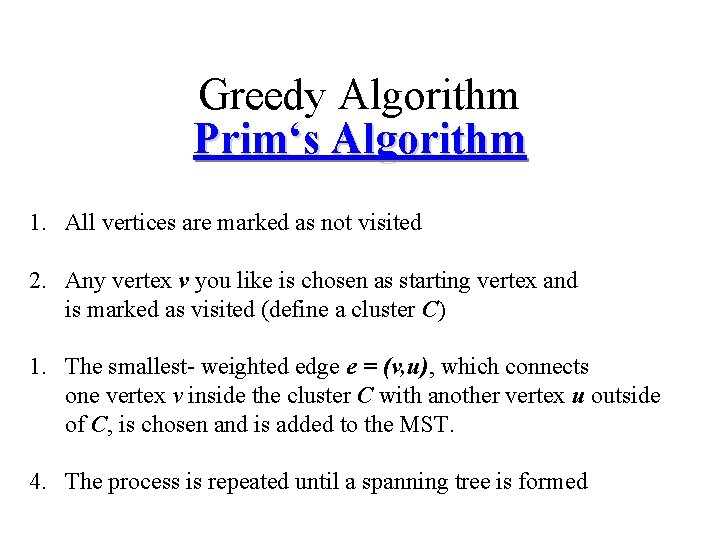
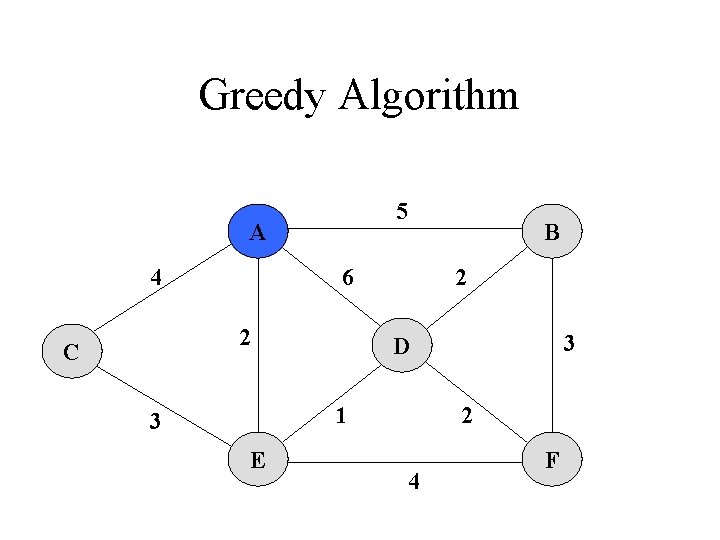
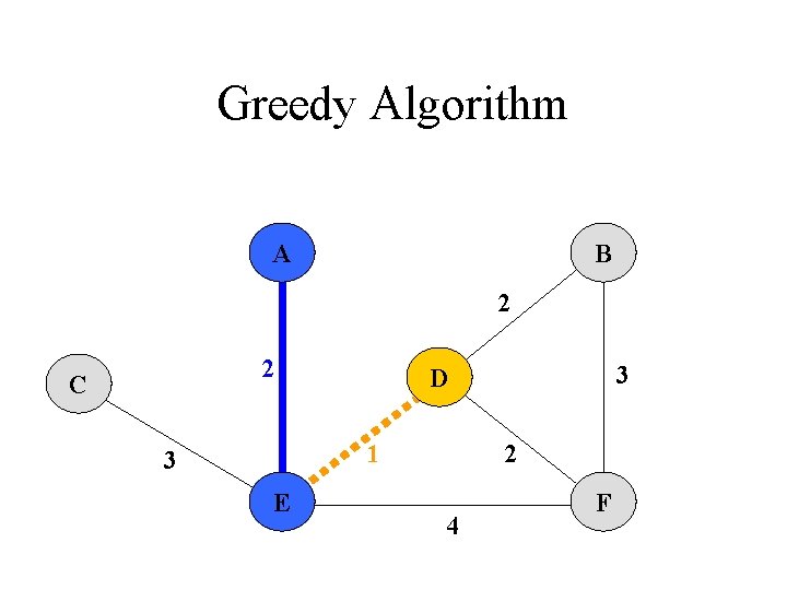
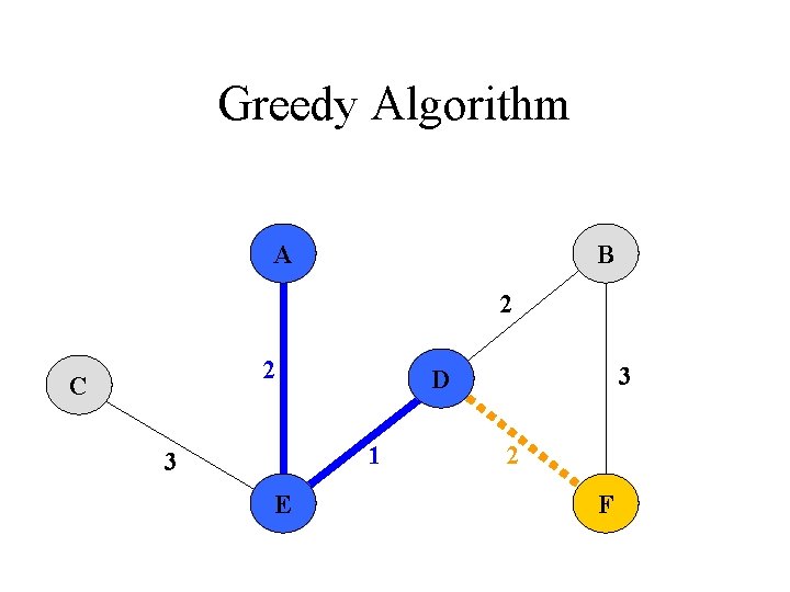
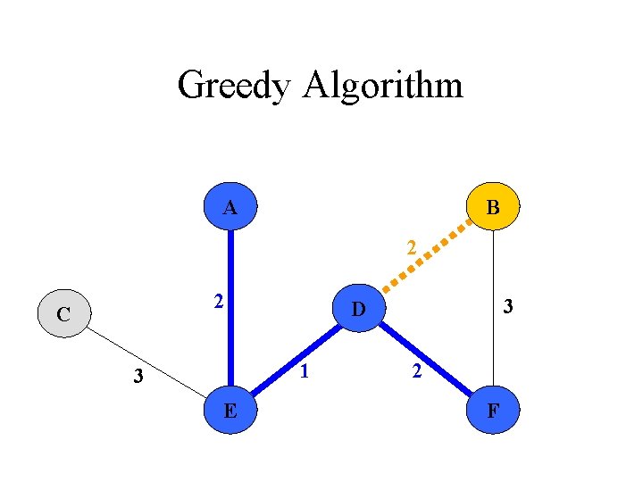
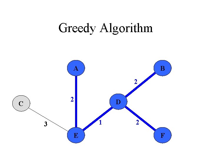
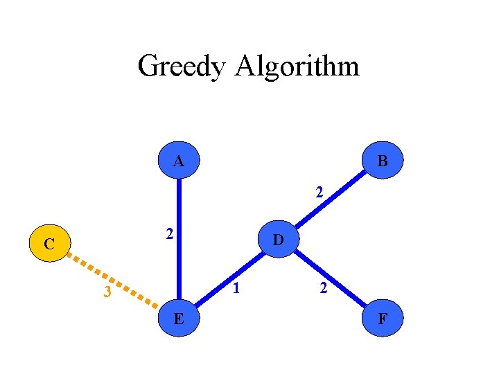
Greedy Algorithm Prim‘s Algorithm 1. All vertices are marked as not visited 2. Any vertex v you like is chosen as starting vertex and is marked as visited (define a cluster C) 1. The smallest- weighted edge e = (v, u), which connects one vertex v inside the cluster C with another vertex u outside of C, is chosen and is added to the MST. 4. The process is repeated until a spanning tree is formed

Greedy Algorithm 5 A 4 6 2 C B 2 1 3 E 3 D 2 4 F

Greedy Algorithm 5 A 4 6 2 C B 2 1 3 E 3 D 2 4 F

Greedy Algorithm We could delete these edges because of Dijkstra‘s label D[u] for each vertex outside of the cluster 5 A 4 6 2 C B 2 1 3 E 3 D 2 4 F

Greedy Algorithm A B 2 2 C 1 3 E 3 D 2 4 F

Greedy Algorithm A B 2 2 C 1 3 E 3 D 2 F

Greedy Algorithm A B 2 2 C 1 3 E 3 D 2 F

Greedy Algorithm A B 2 2 C D 1 3 E 2 F

Greedy Algorithm A B 2 2 C D 1 3 E 2 F

Greedy Algorithm minimum- spanning tree A B 2 2 C D 1 3 E 2 F

Greedy Algorithm Crucial Fact about MSTs Running time: O ( m log n ) By implementing queue Q as a heap, Q could be initialized in O ( m ) time and a vertex could be extracted in each iteration in O ( log n ) time

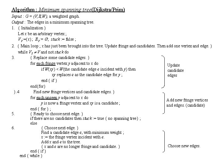
Algorithm : Minimum spanning tree(Dijkstra/Prim) Input : G = (V, E, W), a weighted graph. Output : The edges in a minimum spanning tree. 1. { Initialization } Let x be an arbitrary vertex ; VT: ={x}; ET: = Ø; stuck : = false ; 2. { Main loop ; x has just been brought into the tree. Update fringe and candidates. Then add one vertex and edge. } while VT V and not stuck do 3. { Replace some candidate edges. } for each fringe vertex y adjacent to x do Update if W(xy) < W(the candidate edge e incident with y) then candidate xy replaces e as the candidate edge for y ; edges end { if } end{for} }. 4 Find new fringe vertices and candidate edges. } for each unseen y adjacent to x do Add new fringe vertices y is now a fringe vertex and xy is a candidate ; and edges. (candidate) end { for } ; 5. { Ready to choose next edge. } if there are no candidates then stuck : = true { no spanning tree} ; else 6. { Choose next edge. } Find a candidate edge e, with minimum weight ; x : = the fringe vertex incident with e. Add x and e to the tree. Choose new edges. { x and e are no longer fringe and candidate. } end { if } end { while }

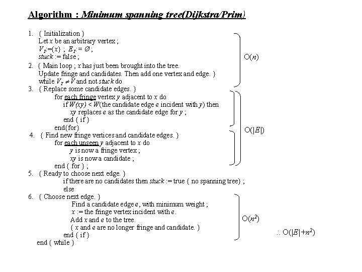
Algorithm : Minimum spanning tree(Dijkstra/Prim) 1. { Initialization } Let x be an arbitrary vertex ; VT: ={x} ; ET: = Ø ; stuck : = false ; O(n) 2. { Main loop ; x has just been brought into the tree. Update fringe and candidates. Then add one vertex and edge. } while VT V and not stuck do 3. { Replace some candidate edges. } for each fringe vertex y adjacent to x do if W(xy) < W(the candidate edge e incident with y) then xy replaces e as the candidate edge for y ; end { if } end{for} O(|E|) 4. { Find new fringe vertices and candidate edges. } for each unseen y adjacent to x do y is now a fringe vertex ; xy is now a candidate ; end { for } ; 5. { Ready to choose next edge. } if there are no candidates then stuck : = true { no spanning tree} ; else 6. { Choose next edge. } Find a candidate edge e, with minimum weight ; x : = the fringe vertex incident with e. O(n 2) Add x and e to the tree. { x and e are no longer fringe and candidate. } end { if } end { while } O(|E|+n 2)

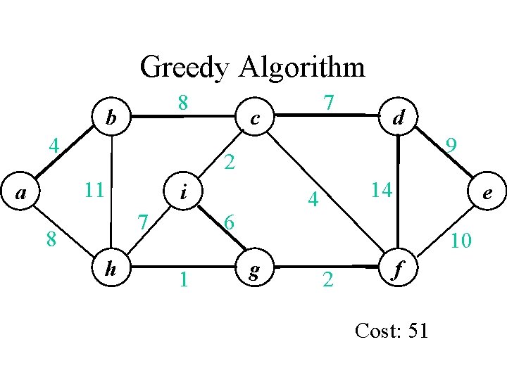
Greedy Algorithm 8 b 4 c d 9 2 11 a 7 i 7 8 h 4 6 1 14 e 10 g 2 f Cost: 51

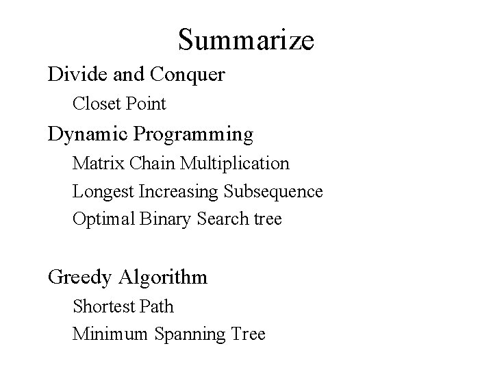
Summarize Divide and Conquer Closet Point Dynamic Programming Matrix Chain Multiplication Longest Increasing Subsequence Optimal Binary Search tree Greedy Algorithm Shortest Path Minimum Spanning Tree

Final Examination 10 questions, 120 points (selects 7 questions) Part I (1 -3) Running Time, Definition Part II (4 -8) select 3 from 5 Part III (9 -10) Unseen Start from After midterm lecture !!