Recursion and Dynamic Programming Recursive thinking Recursion is

Recursion and Dynamic Programming

Recursive thinking… • Recursion is a method where the solution to a problem depends on solutions to smaller instances of the same problem – or, in other words, a programming technique in which a method can call itself to solve a problem.

Example: Factorial • The factorial for any positive integer n, written n!, is defined to be the product of all integers between 1 and n inclusive n!= nx(n− 1) x(n− 2)x. . . x 1

Non-recursive solution

Recursive factorial

Key Features of Recursions • Simple solution for a few cases • Recursive definition for other values – Computation of large N depends on smaller N • Can be naturally expressed in a function that calls itself – Loops are many times an alternative

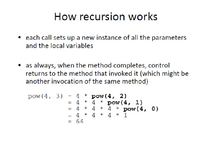
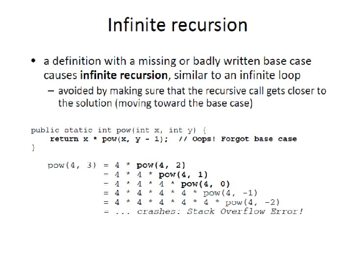
Recursive power example • Write method pow that takes integers x and y as parameters and returns xy. xy = x * x *. . . * x (y times, in total) An iterative solution:

Recursive power function • Another way to define the power function:

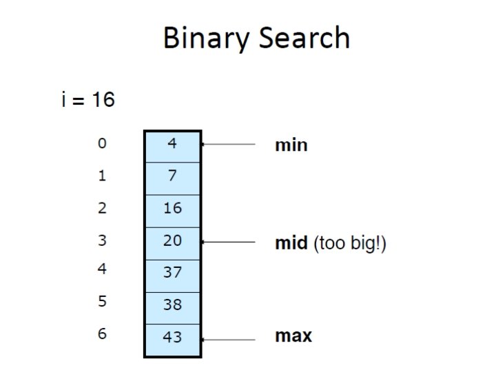
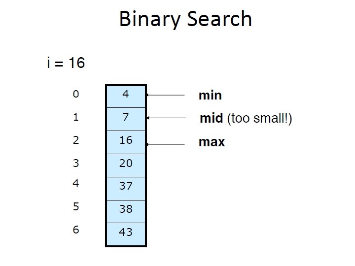
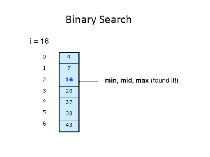
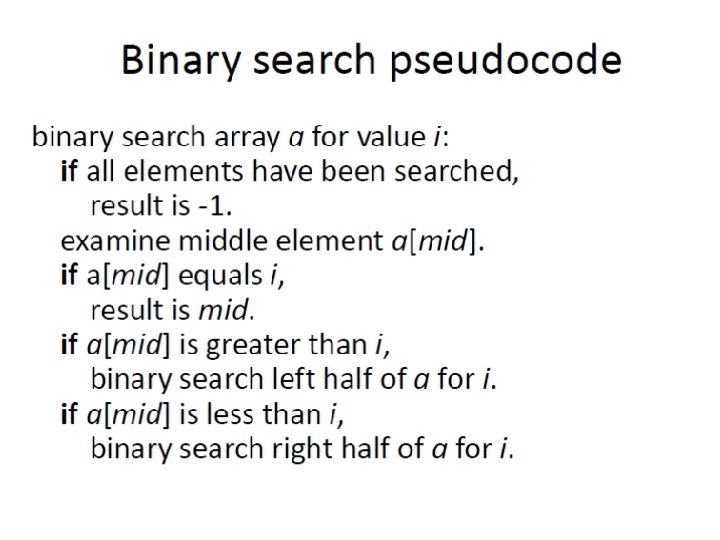
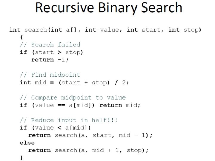
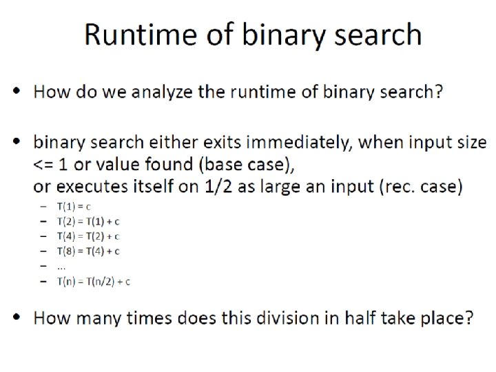
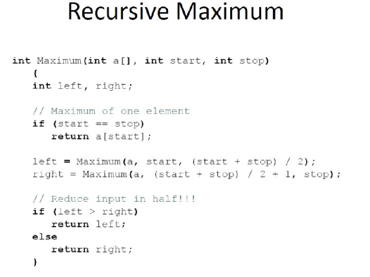
Divide-and-conquer Algorithms Divide-and-conquer algorithm: a means for solving a problem that • first separates the main problem into 2 or more smaller problems, • Then solves each of the smaller problems, • Then uses those sub-solutions to solve the original problem 1: "divide" the problem up into pieces 2: "conquer" each smaller piece 3: (if necessary) combine the pieces at the end to produce the overall solution Binary search is one such algorithm

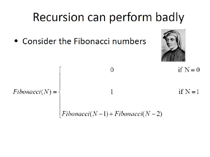
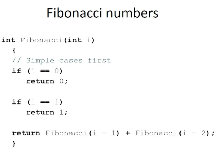
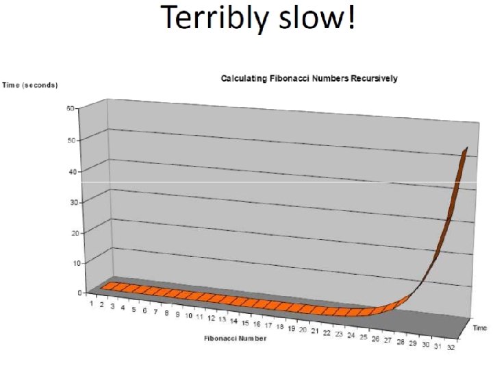
Recursion can perform badly • Fibonacci numbers The higher up in the sequence, the closer two consecutive "Fibonacci numbers" of the sequence divided by each other will approach the golden ratio (approximately 1 : 1. 618)

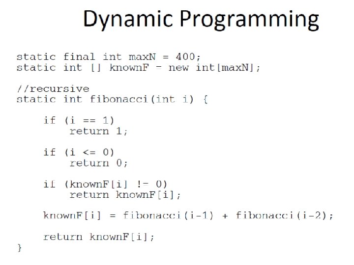
What is going on? • Certain quantities are recalculated far too many times! • Need to avoid recalculation… – Ideally, calculate each unique quantity once

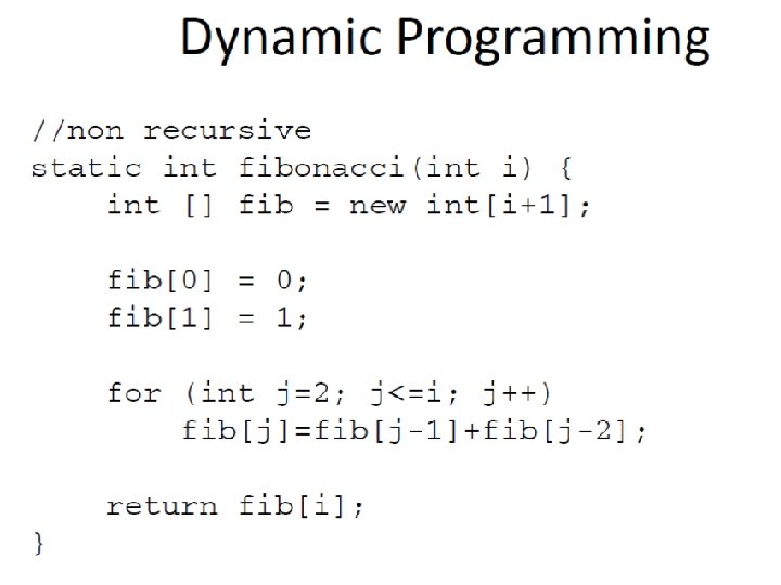
Dynamic programming Time: linear

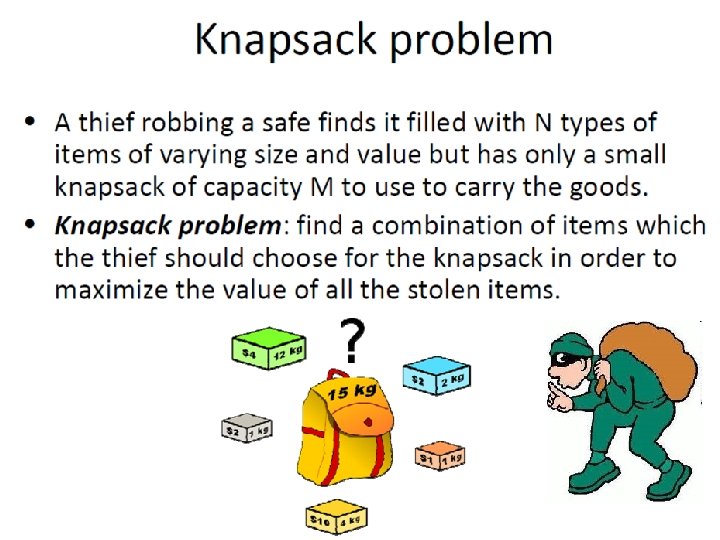
The Knapsack problem Size Val 17 24 18 17 24 19 20 23 21 17 An instance of the knapsack problem consists of a knapsack capacity and a set of items of varying size (horizontal dimension) and value (vertical dimension). This figure shows four different ways to fill a knapsack of size 17, two of which lead to the highest possible total value of 24.

Recursive solution • Assume that item i is selected to be in the knapsack • Find what would be the optimal value assuming optimization for all remaining items • Requires solving a smaller knapsack problem

The Knapsack problem We have an array of N items of type Item. For each possible item, we calculate (recursively) the maximum value that we could achieve by including that item, then take the maximum of all those values. static class Item { int size; int val; } static int knap(int cap) { int i, space, max, t; for (i = 0, max = 0; i < N; i++) if ((space = cap-items[i]. size) >= 0) if ((t = knap(space) + items[i]. val) > max) max = t; return max; }

The Knapsack problem The number in each node represents the remaining capacity in the knapsack. The algorithm suffers the same basic problem of exponential performance due to massive recomputation for overlapping subproblems that we considered in computing Fibonacci numbers Exponential time !!

The Knapsack problem static int knap(int cap) { int i, space, maxi = 0, t; if (max. Known[cap] != unknown) return max. Known[cap]; for (i = 0, max = 0; i < N; i++) if ((space = cap-items[i]. size) >= 0) if ((t = knap(space) + items[i]. val) > max) { max = t; maxi = i; } } max. Known[cap] = max; item. Known[cap] = items[maxi]; return max;

The Knapsack problem

Time consideration • The running time is at most the running time to evaluate the function for all arguments less than or equal to the given argument • Time ~NM (N: types of items, M: maximum total value of items)

Bottom-up and Top-down • In bottom-up – We precompute all possible values • In top-down – We use already computed values (on demand) • Generally top down preferable – Closer to a natural solution – Order of computing simple – We may not need to solve all subproblems