DREAM IDEA PLAN IMPLEMENTATION 1 LinearControlSystems Present to

DREAM IDEA PLAN IMPLEMENTATION 1

Linear-Control-Systems Present to: Amirkabir University of Technology (Tehran Polytechnic) & Semnan University Dr. Kourosh Kiani Email: kkiani 2004@yahoo. com Email: Kourosh. kiani@aut. ac. ir Web: aut. ac. com 2

Lecture 15 3

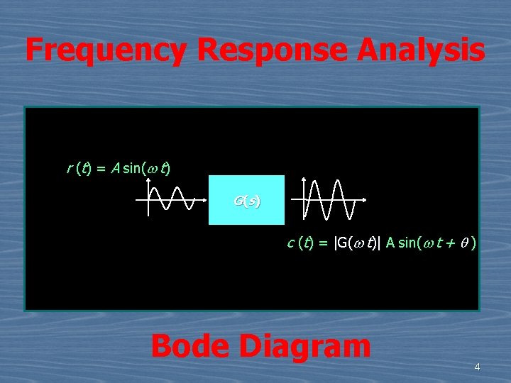
Frequency Response Analysis r (t) = A sin(w t) G(s ) c (t) = |G(w t)| A sin(w t + q ) Bode Diagram 4

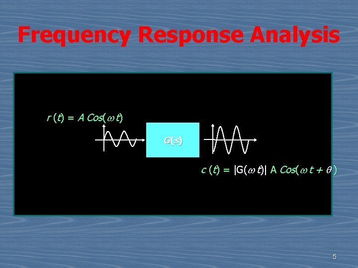
Frequency Response Analysis r (t) = A Cos(w t) G(s ) c (t) = |G(w t)| A Cos(w t + q ) 5

A Perspective on the Frequency-Response Design Method The design of feedback control systems in industry is probably accomplished using frequency-response methods more than any other. Advantages of frequency-response design: -It provides good designs in the face of uncertainty in the plant model -Experimental information can be used for design purposes. Raw measurements of the output amplitude and phase of a plant undergoing a sinusoidal input excitation are sufficient to design a suitable feedback control. -No intermediate processing of the data (such as finding poles and zeros) is required to arrive at the system model. 6

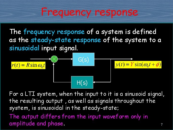
Frequency response The frequency response of a system is defined as the steady-state response of the system to a sinusoidal input signal. G(s) H(s) For a LTI system, when the input to it is a sinusoid signal, the resulting output , as well as signals throughout the system, is sinusoidal in the steady-state; The output differs from the input waveform only in amplitude and phase. 7

Frequency Response of a System n n Thus the output is equal to the input sinusoid multiplied by the gain, |G(jw)| and shifted by the angle, /G(jw). These characteristics can be obtained by substituting, s = jw into G(s), or from measurements on the physical system. c(t) = |G(wt)| A sin(wt + q ) r(t) = A sin(wt) G ( s) 8

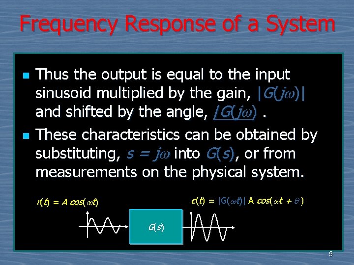
Frequency Response of a System n n Thus the output is equal to the input sinusoid multiplied by the gain, |G(jw)| and shifted by the angle, /G(jw). These characteristics can be obtained by substituting, s = jw into G(s), or from measurements on the physical system. c(t) = |G(wt)| A cos(wt + q ) r(t) = A cos(wt) G ( s) 9

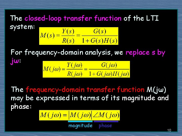
The closed-loop transfer function of the LTI system: For frequency-domain analysis, we replace s by jω: The frequency-domain transfer function M(jω) may be expressed in terms of its magnitude and phase: magnitude phase 10

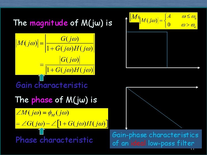
The magnitude of M(jω) is Gain characteristic The phase of M(jω) is Phase characteristic Gain-phase characteristics of an ideal low-pass filter 11

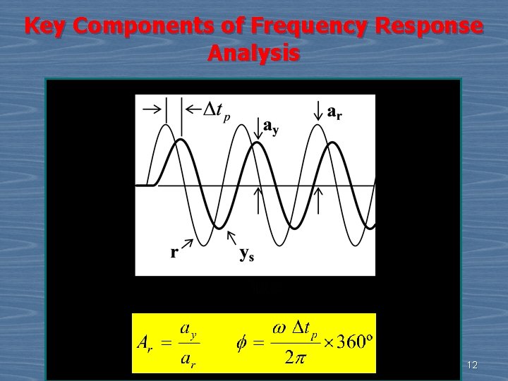
Key Components of Frequency Response Analysis 12

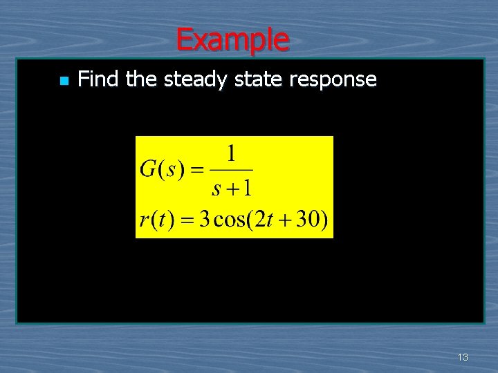
Example n Find the steady state response 13

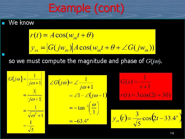
Example (cont) n n We know so we must compute the magnitude and phase of G(jw). 14

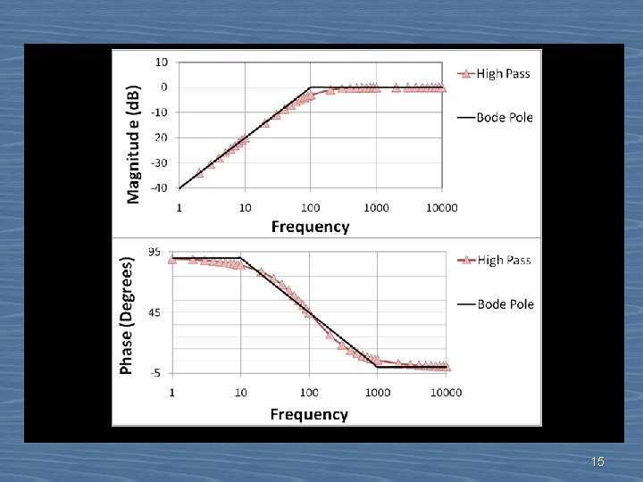
15

16

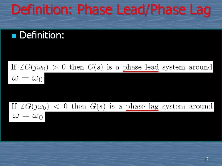
Definition: Phase Lead/Phase Lag n Definition: 17

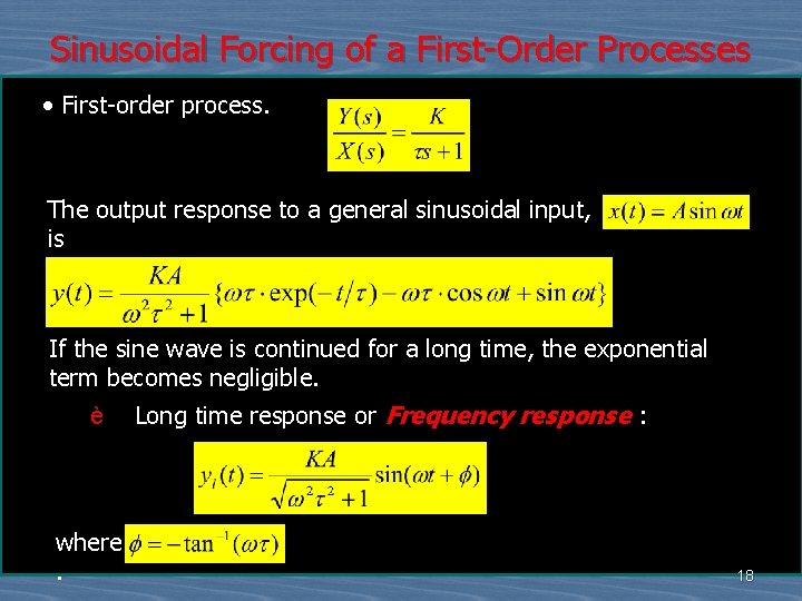
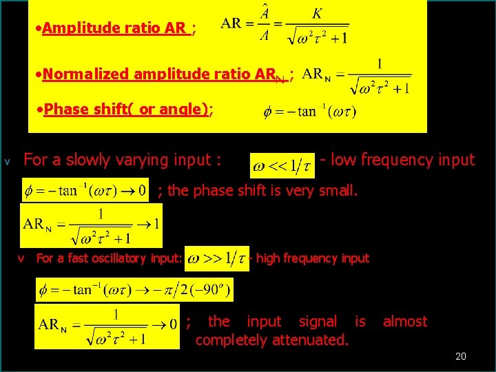
Sinusoidal Forcing of a First-Order Processes • First-order process. The output response to a general sinusoidal input, is If the sine wave is continued for a long time, the exponential term becomes negligible. è Long time response or Frequency response : where . 18

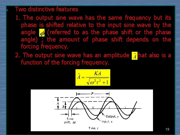
v Two distinctive features 1. The output sine wave has the same frequency but its phase is shifted relative to the input sine wave by the angle (referred to as the phase shift or the phase angle) ; the amount of phase shift depends on the forcing frequency. 2. The output sine wave has an amplitude that also is a function of the forcing frequency. 19

• Amplitude ratio AR ; • Normalized amplitude ratio ARN ; • Phase shift( or angle); v For a slowly varying input : - low frequency input ; the phase shift is very small. v For a fast oscillatory input: - high frequency input ; the input signal is almost completely attenuated. 20

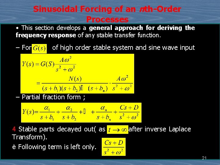
Sinusoidal Forcing of an nth-Order Processes • This section develops a general approach for deriving the frequency response of any stable transfer function. – For of high order stable system and sine wave input – Partial fraction form ; 4 Stable parts decayed out( as after inverse Laplace Transform). è Following term is left only. 21

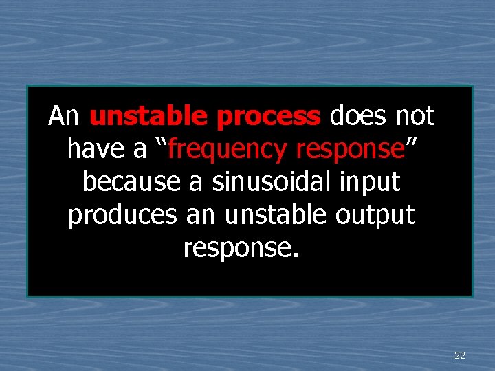
An unstable process does not have a “frequency response” because a sinusoidal input produces an unstable output response. 22

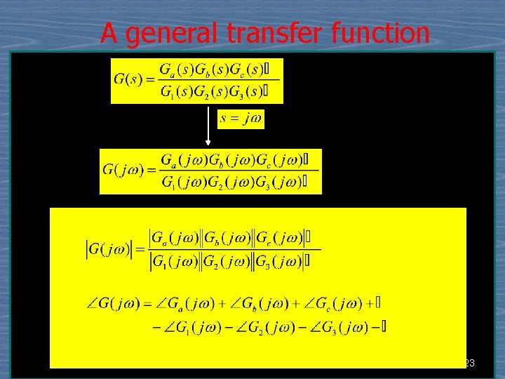
A general transfer function 23

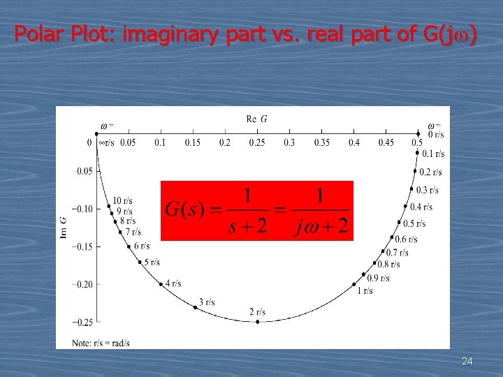
Polar Plot: imaginary part vs. real part of G(jw) 24

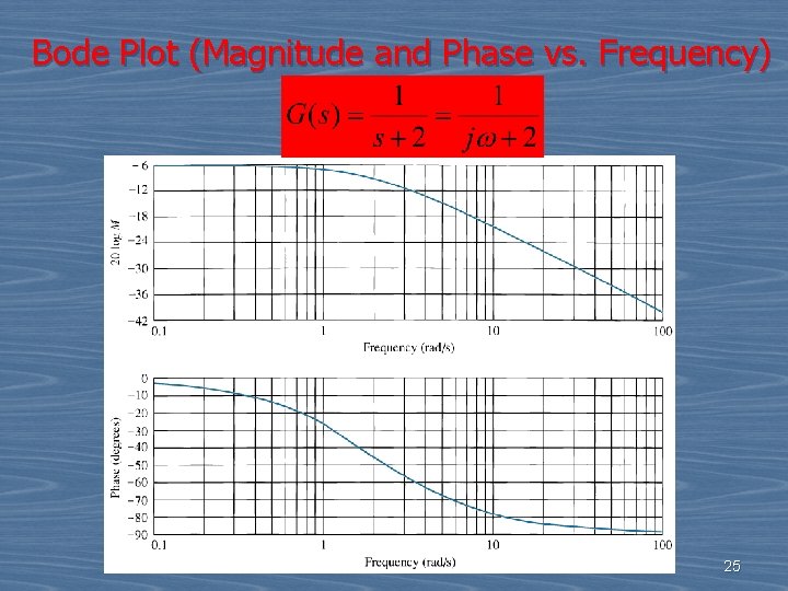
Bode Plot (Magnitude and Phase vs. Frequency) 25

Bode diagram 26

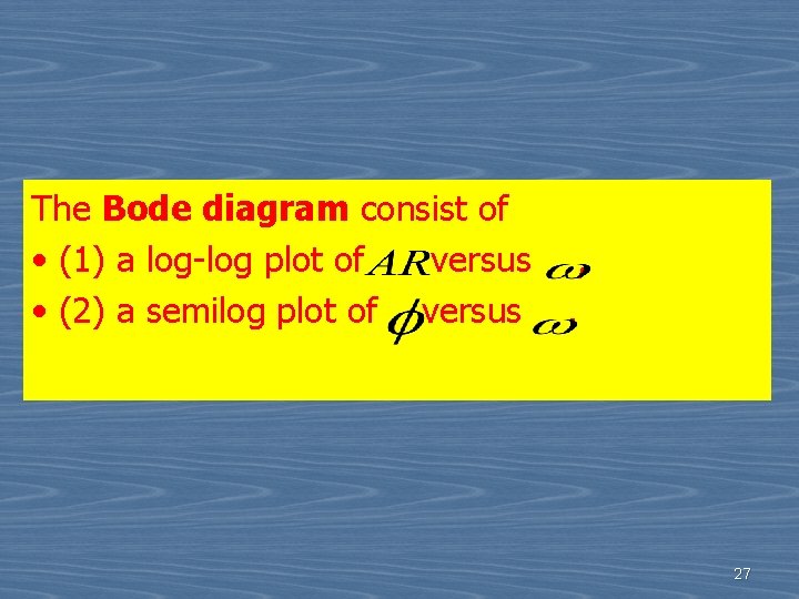
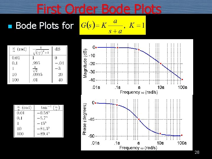
The Bode diagram consist of • (1) a log-log plot of versus , • (2) a semilog plot of versus . 27

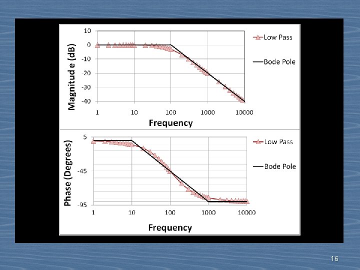
First Order Bode Plots n Bode Plots for 28

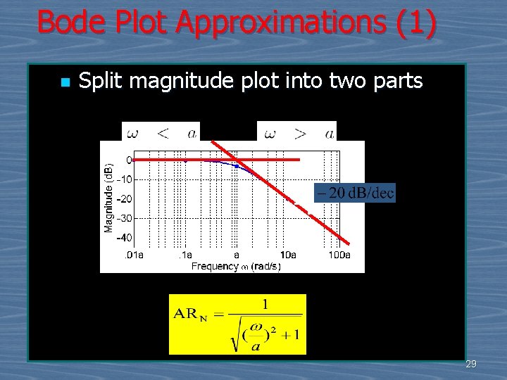
Bode Plot Approximations (1) n Split magnitude plot into two parts 29

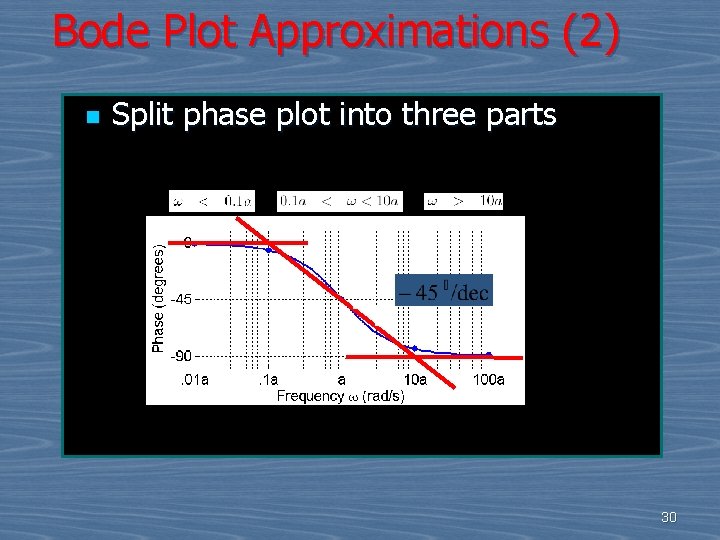
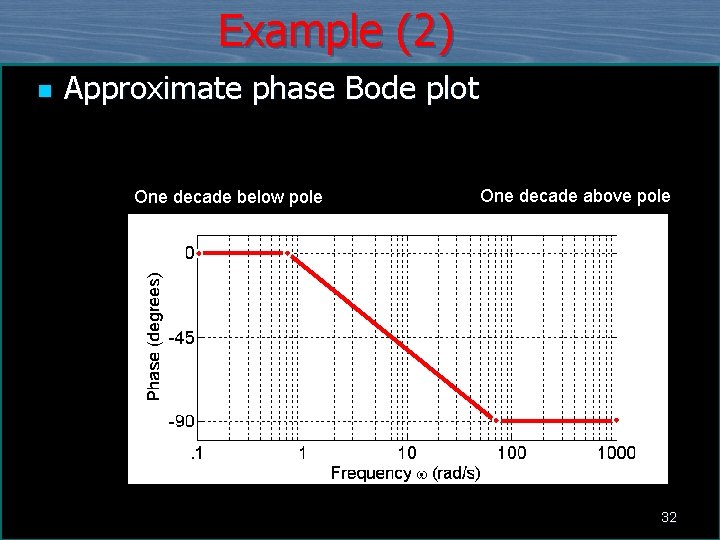
Bode Plot Approximations (2) n Split phase plot into three parts 30

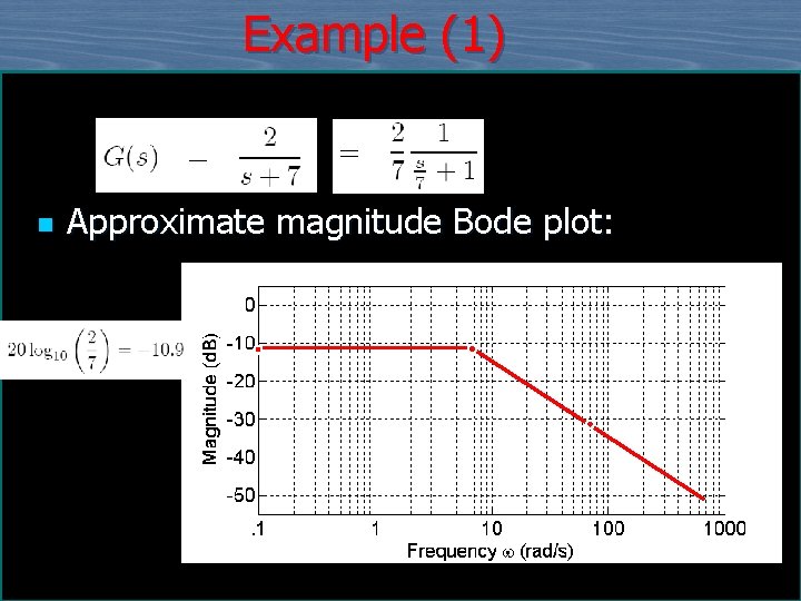
Example (1) n Approximate magnitude Bode plot:

Example (2) n Approximate phase Bode plot One decade below pole One decade above pole 32

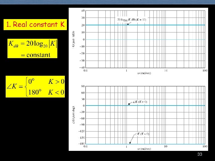
1. Real constant K 33

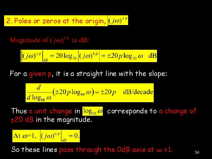
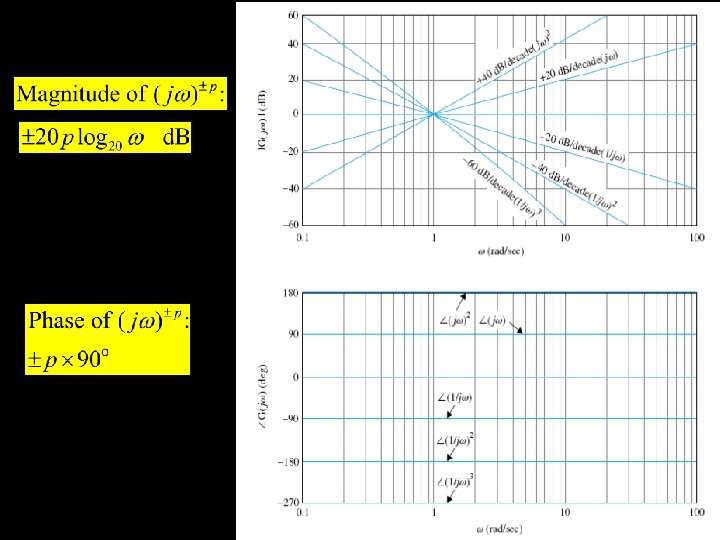
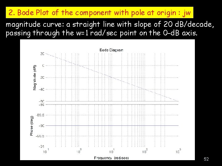
2. Poles or zeros at the origin, For a given p, it is a straight line with the slope: Thus a unit change in ± 20 d. B in the magnitude. corresponds to a change of So these lines pass through the 0 d. B axis at ω =1. 34

35

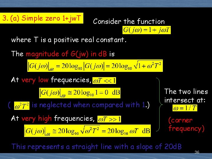
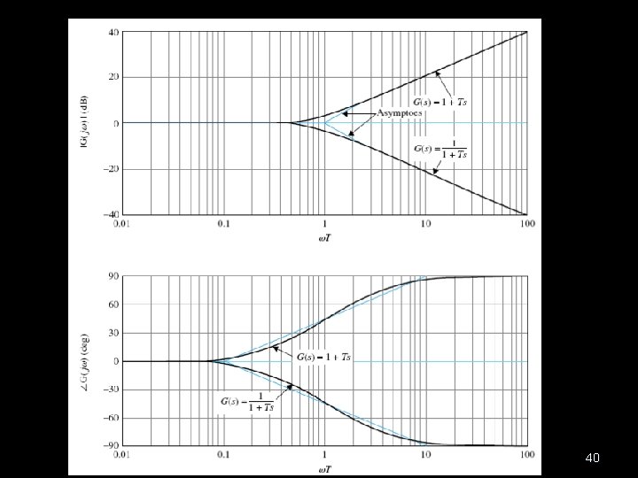
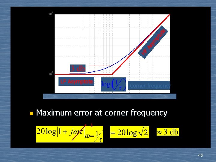
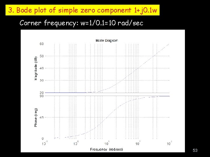
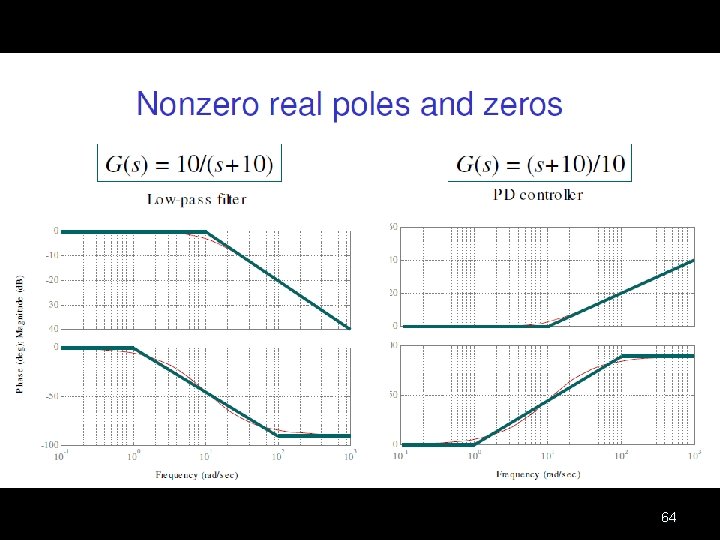
3. (a) Simple zero 1+jw. T Consider the function where T is a positive real constant. The magnitude of G(jw) in d. B is At very low frequencies, ( is neglected when compared with 1. ) At very high frequencies, The two lines intersect at: (corner frequency) This represents a straight line with a slope of 20 d. B 36

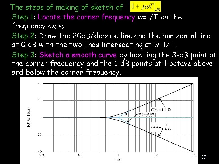
The steps of making of sketch of Step 1: Locate the corner frequency w=1/T on the frequency axis; Step 2: Draw the 20 d. B/decade line and the horizontal line at 0 d. B with the two lines intersecting at w=1/T. Step 3: Sketch a smooth curve by locating the 3 -d. B point at the corner frequency and the 1 -d. B points at 1 octave above and below the corner frequency. 37

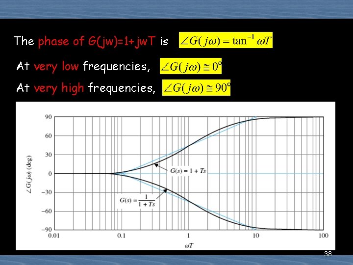
The phase of G(jw)=1+jw. T is At very low frequencies, At very high frequencies, 38

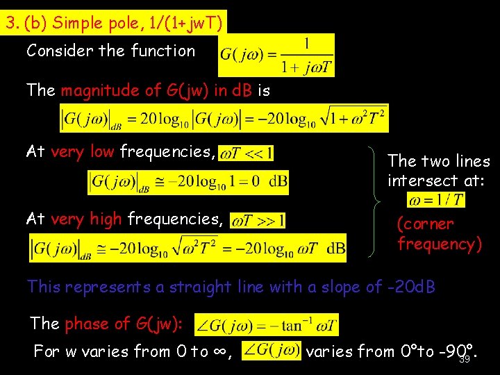
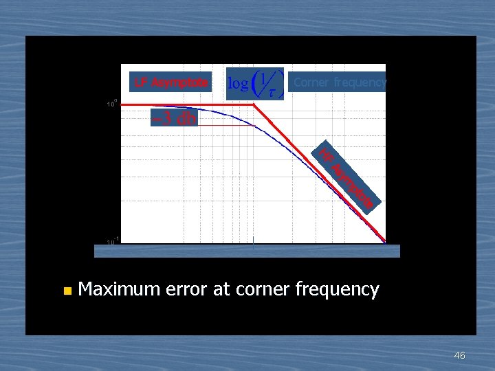
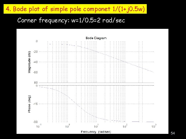
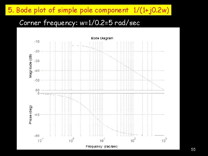
3. (b) Simple pole, 1/(1+jw. T) Consider the function The magnitude of G(jw) in d. B is At very low frequencies, At very high frequencies, The two lines intersect at: (corner frequency) This represents a straight line with a slope of -20 d. B The phase of G(jw): For w varies from 0 to ∞, varies from 0°to -90°. 39

40

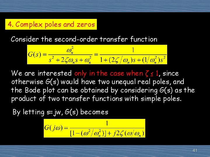
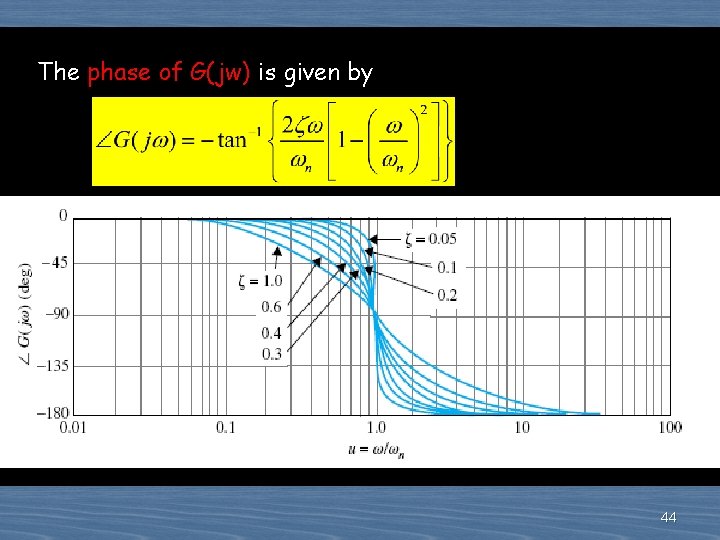
4. Complex poles and zeros Consider the second-order transfer function We are interested only in the case when ζ ≤ 1, since otherwise G(s) would have two unequal real poles, and the Bode plot can be obtained by considering G(s) as the product of two transfer functions with simple poles. By letting s=jw, G(s) becomes 41

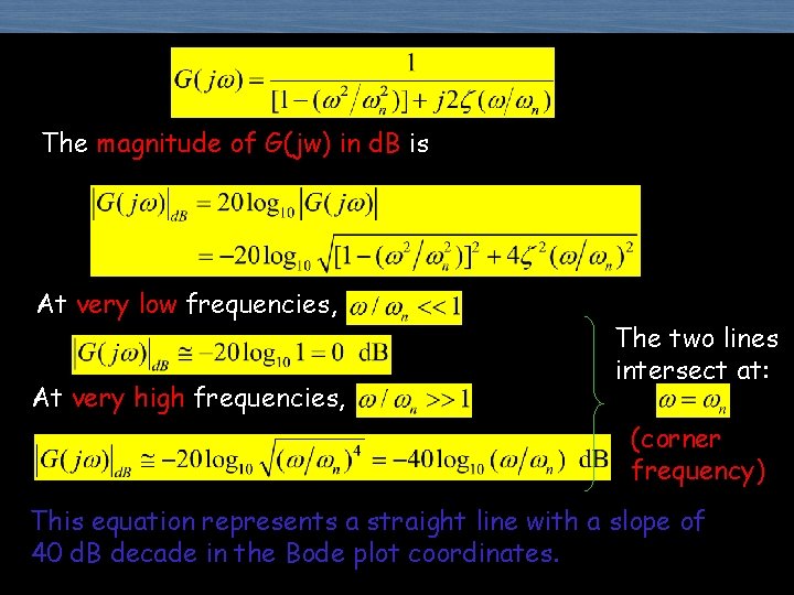
The magnitude of G(jw) in d. B is At very low frequencies, At very high frequencies, The two lines intersect at: (corner frequency) This equation represents a straight line with a slope of 40 d. B decade in the Bode plot coordinates.

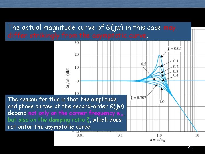
The actual magnitude curve of G(jw) in this case may differ strikingly from the asymptotic curve. The reason for this is that the amplitude and phase curves of the second-order G(jw) depend not only on the corner frequency wn, but also on the damping ratio ζ, which does not enter the asymptotic curve. 43

The phase of G(jw) is given by 44

ym pt ot e A s HF LF Asymptote n Corner frequency Maximum error at corner frequency 1 45

LF Asymptote Corner frequency e ot pt m sy A HF n Maximum error at corner frequency 46

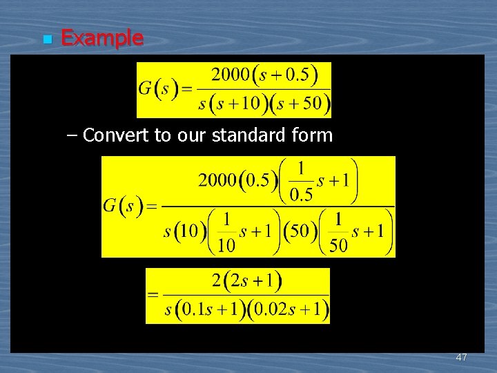
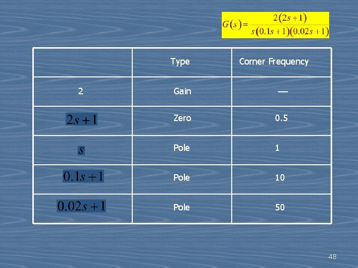
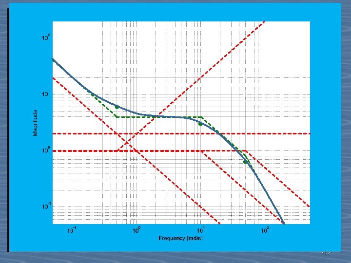
n Example – Convert to our standard form 47

Type 2 Corner Frequency Gain –– Zero 0. 5 Pole 10 Pole 50 48

49

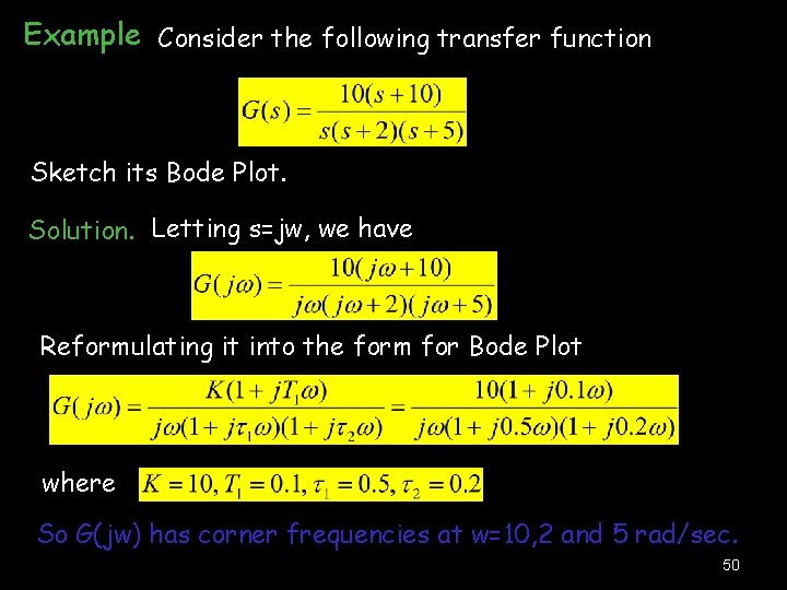
Example Consider the following transfer function Sketch its Bode Plot. Solution. Letting s=jw, we have Reformulating it into the form for Bode Plot where So G(jw) has corner frequencies at w=10, 2 and 5 rad/sec. 50

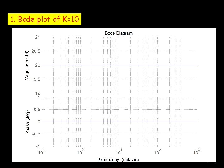
1. Bode plot of K=10 51

2. Bode Plot of the component with pole at origin : jw magnitude curve: a straight line with slope of 20 d. B/decade, passing through the w=1 rad/sec point on the 0 -d. B axis. 52

3. Bode plot of simple zero component 1+j 0. 1 w Corner frequency: w=1/0. 1=10 rad/sec 53

4. Bode plot of simple pole componet 1/(1+j 0. 5 w) Corner frequency: w=1/0. 5=2 rad/sec 54

5. Bode plot of simple pole component 1/(1+j 0. 2 w) Corner frequency: w=1/0. 2=5 rad/sec 55

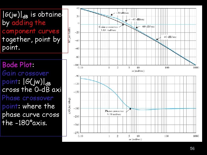
|G(jw)|d. B is obtained by adding the component curves together, point by point. Bode Plot: Gain crossover point: |G(jw)|d. B cross the 0 -d. B axis Phase crossover point: where the phase curve cross the -180°axis. 56

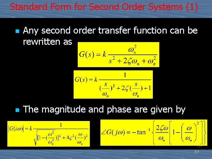
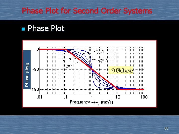
Standard Form for Second Order Systems (1) n n Any second order transfer function can be rewritten as The magnitude and phase are given by 57

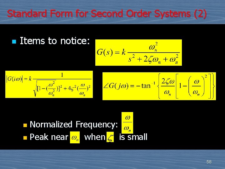
Standard Form for Second Order Systems (2) n Items to notice: Normalized Frequency: n Peak near when is small n 58

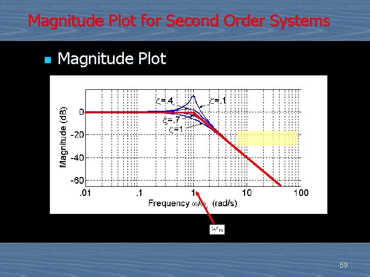
Magnitude Plot for Second Order Systems n Magnitude Plot 59

Phase Plot for Second Order Systems Phase Plot Phase (deg) n 60

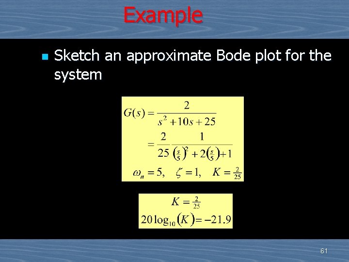
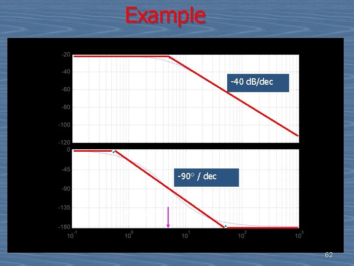
Example n Sketch an approximate Bode plot for the system 61

Example -40 d. B/dec -90° / dec wn = 5 rad/s 62

Draw Bode diagram using Mat. Lab num. G = [2]; % Define numerator of G(s). den. G = [1 10 25]; % Define denominator of G(s). G = tf(num. G, den. G) % Create and display G(s). bode(G); % Draw Bode diagram. 63

64

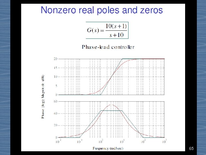
65

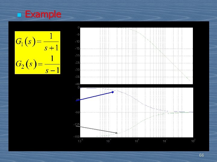
n Example 66

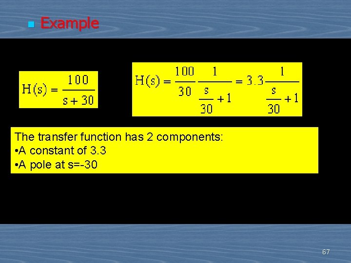
n Example The transfer function has 2 components: • A constant of 3. 3 • A pole at s=-30 67

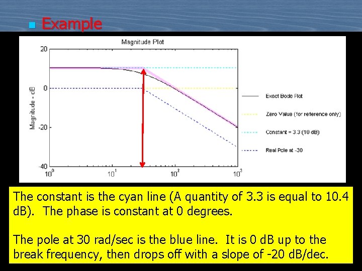
n Example The constant is the cyan line (A quantity of 3. 3 is equal to 10. 4 d. B). The phase is constant at 0 degrees. The pole at 30 rad/sec is the blue line. It is 0 d. B up to the break frequency, then drops off with a slope of -20 d. B/dec. 68

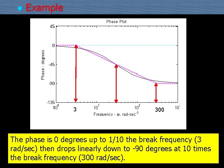
n Example 3 300 The phase is 0 degrees up to 1/10 the break frequency (3 rad/sec) then drops linearly down to -90 degrees at 10 times the break frequency (300 rad/sec). 69

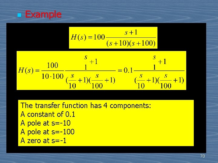
n Example The transfer function has 4 components: A constant of 0. 1 A pole at s=-100 A zero at s=-1 70

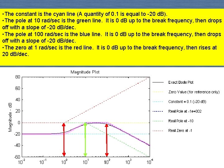
• The constant is the cyan line (A quantity of 0. 1 is equal to -20 d. B). • The pole at 10 rad/sec is the green line. It is 0 d. B up to the break frequency, then drops off with a slope of -20 d. B/dec. • The pole at 100 rad/sec is the blue line. It is 0 d. B up to the break frequency, then drops off with a slope of -20 d. B/dec. • The zero at 1 rad/sec is the red line. It is 0 d. B up to the break frequency, then rises at 20 d. B/dec. 71

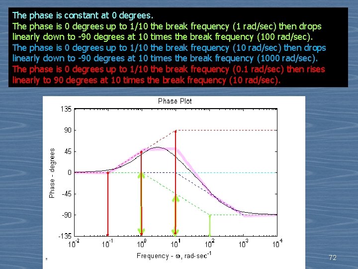
The phase is constant at 0 degrees. The phase is 0 degrees up to 1/10 the break frequency (1 rad/sec) then drops linearly down to -90 degrees at 10 times the break frequency (100 rad/sec). The phase is 0 degrees up to 1/10 the break frequency (10 rad/sec) then drops linearly down to -90 degrees at 10 times the break frequency (1000 rad/sec). The phase is 0 degrees up to 1/10 the break frequency (0. 1 rad/sec) then rises linearly to 90 degrees at 10 times the break frequency (10 rad/sec). 72

Introductory to Complex Numbers APPENDIX of This Lecture

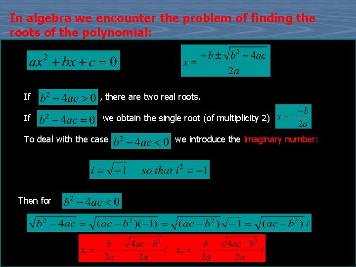
In algebra we encounter the problem of finding the roots of the polynomial: If , there are two real roots. If , we obtain the single root (of multiplicity 2) To deal with the case we introduce the imaginary number: Then for

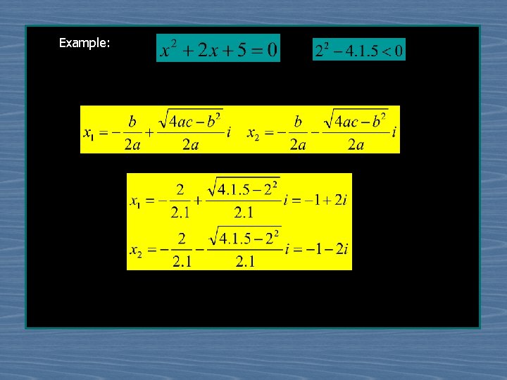
Example:

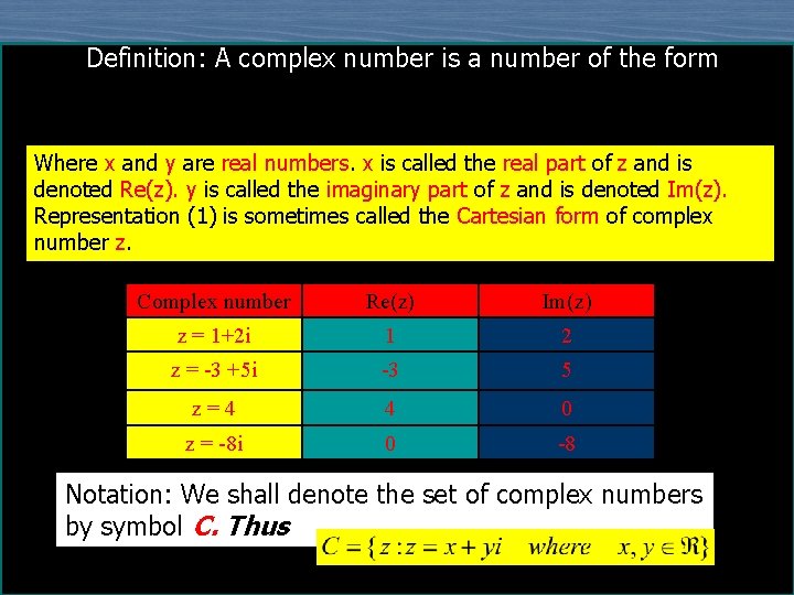
Definition: A complex number is a number of the form Where x and y are real numbers. x is called the real part of z and is denoted Re(z). y is called the imaginary part of z and is denoted Im(z). Representation (1) is sometimes called the Cartesian form of complex number z. Complex number Re(z) Im(z) z = 1+2 i 1 2 z = -3 +5 i -3 5 z=4 4 0 z = -8 i 0 -8 Notation: We shall denote the set of complex numbers by symbol C. Thus

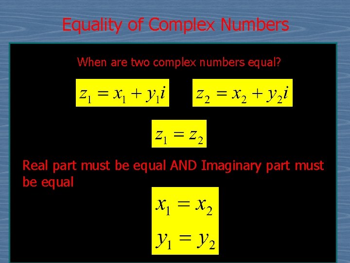
Equality of Complex Numbers When are two complex numbers equal? Real part must be equal AND Imaginary part must be equal

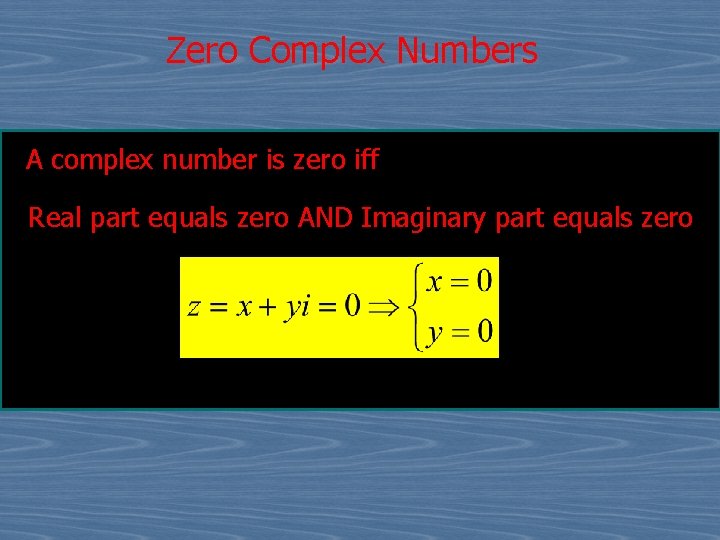
Zero Complex Numbers A complex number is zero iff Real part equals zero AND Imaginary part equals zero

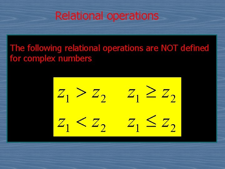
Relational operations The following relational operations are NOT defined for complex numbers

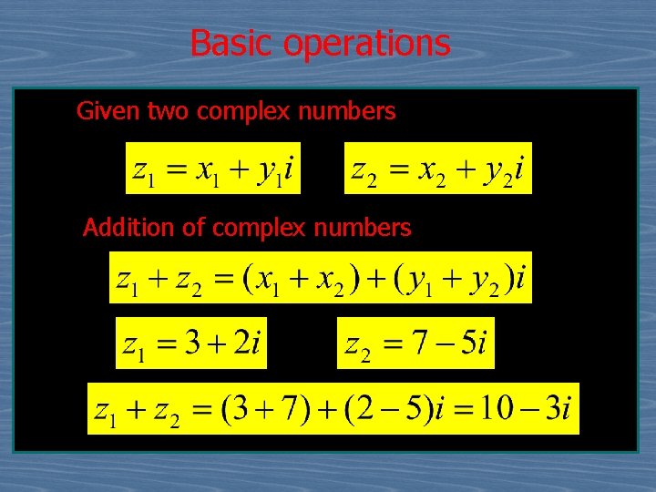
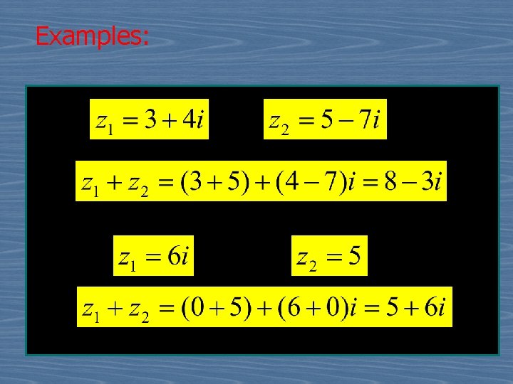
Basic operations Given two complex numbers Addition of complex numbers

Examples:

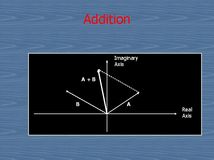
Addition Imaginary Axis A + B B A Real Axis

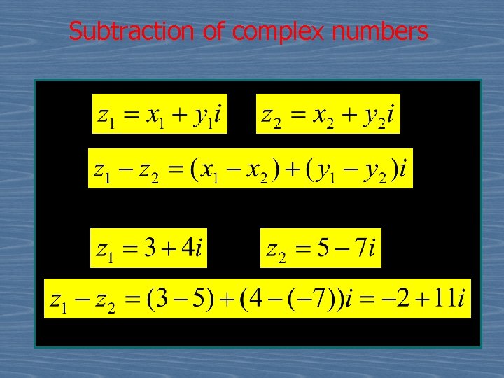
Subtraction of complex numbers

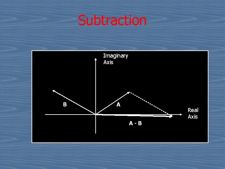
Subtraction Imaginary Axis B A A - B Real Axis

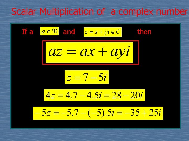
Scalar Multiplication of a complex number If a and then

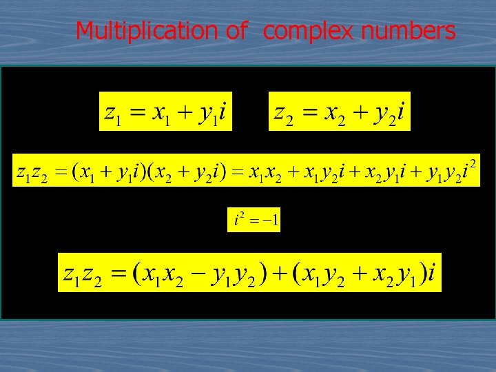
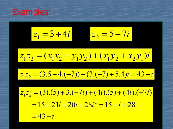
Multiplication of complex numbers

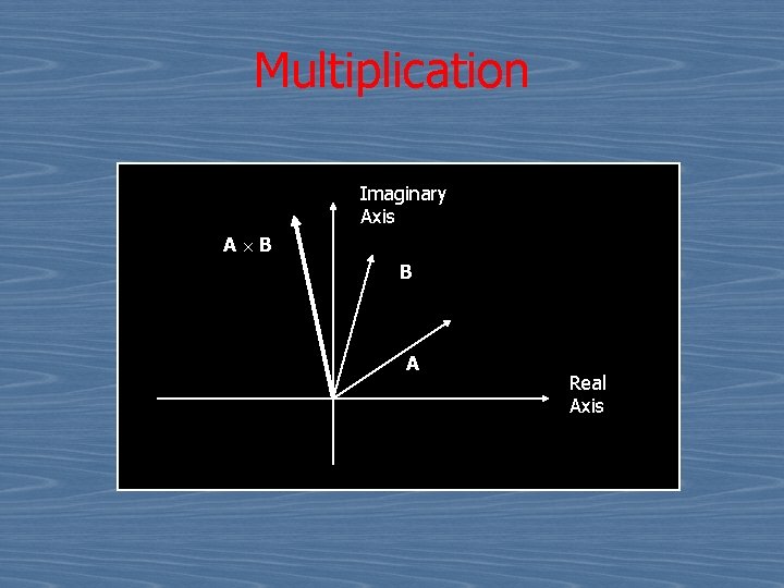
Multiplication Imaginary Axis A B B A Real Axis

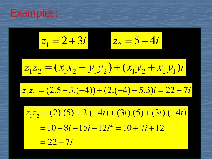
Examples:

Examples:

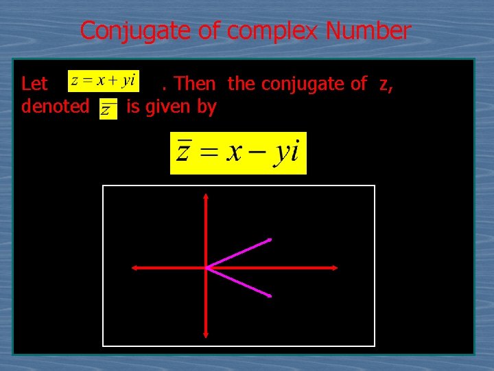
Conjugate of complex Number Let . Then the conjugate of z, denoted is given by y x

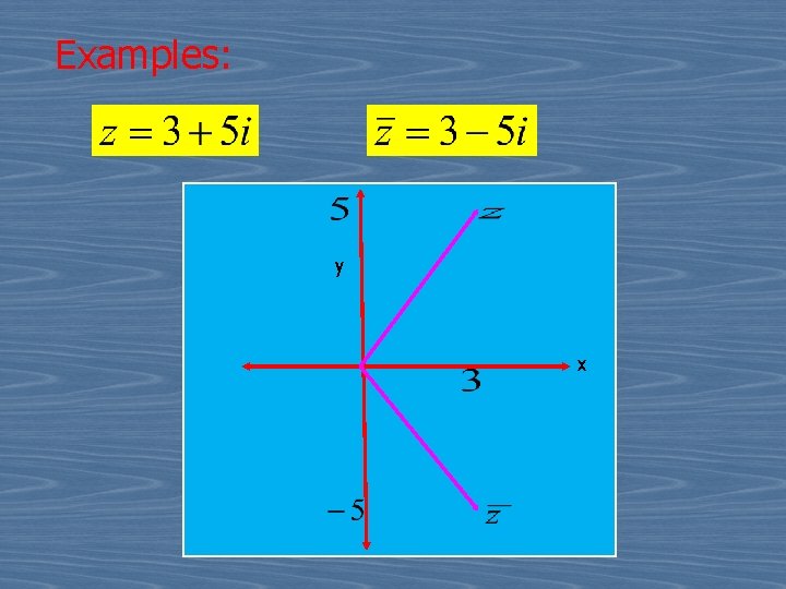
Examples: y x

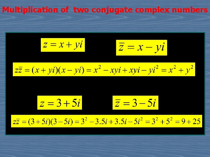
Multiplication of two conjugate complex numbers

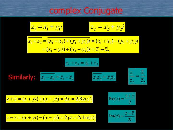
complex Conjugate Similarly:

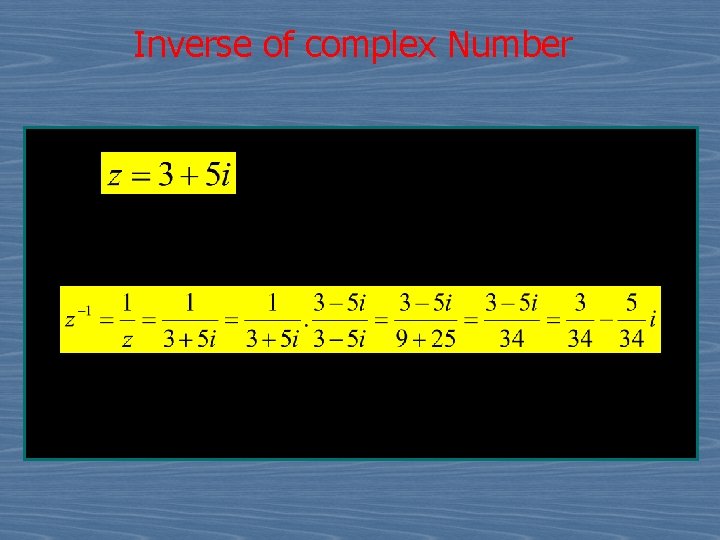
Inverse of complex Number Let

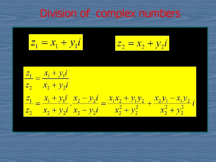
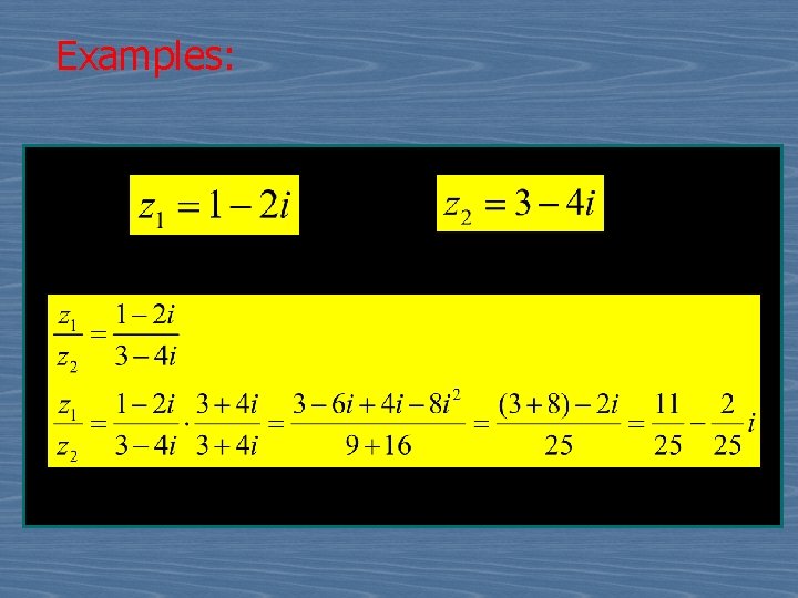
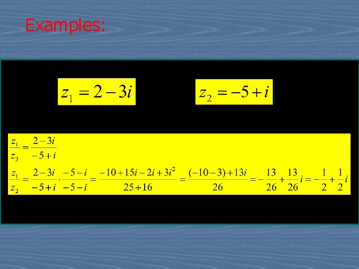
Division of complex numbers

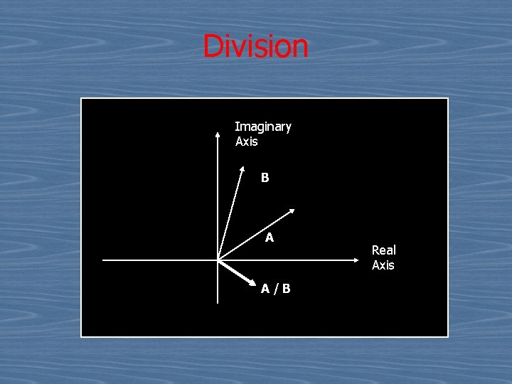
Division Imaginary Axis B A A / B Real Axis

Examples:

Examples:

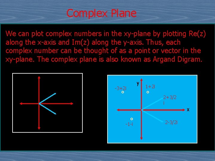
Complex Plane We can plot complex numbers in the xy-plane by plotting Re(z) along the x-axis and Im(z) along the y-axis. Thus, each complex number can be thought of as a point or vector in the xy-plane. The complex plane is also known as Argand Digram. y -3+2 i y 1+2 i 2+3/2 i x x -1 -i 2 -3/2 i

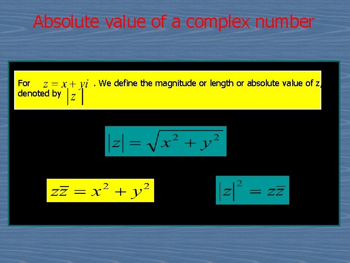
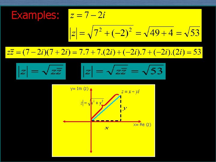
Absolute value of a complex number For . We define the magnitude or length or absolute value of z, denoted by

Examples: y= Im (z) x= Re (z)

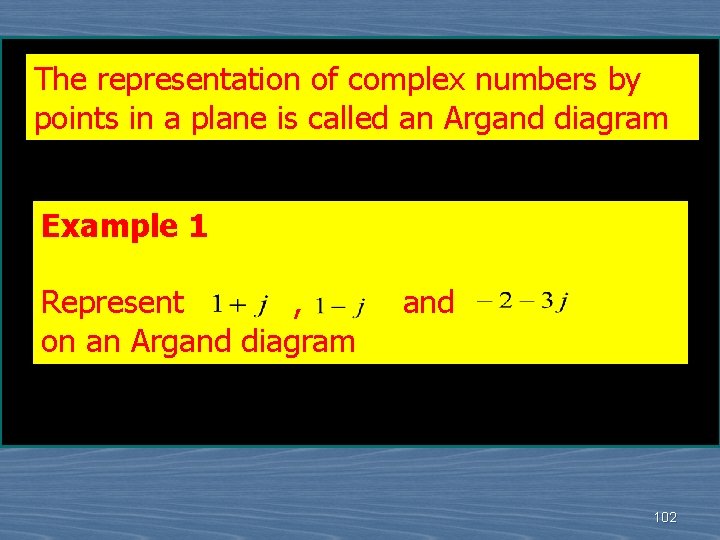
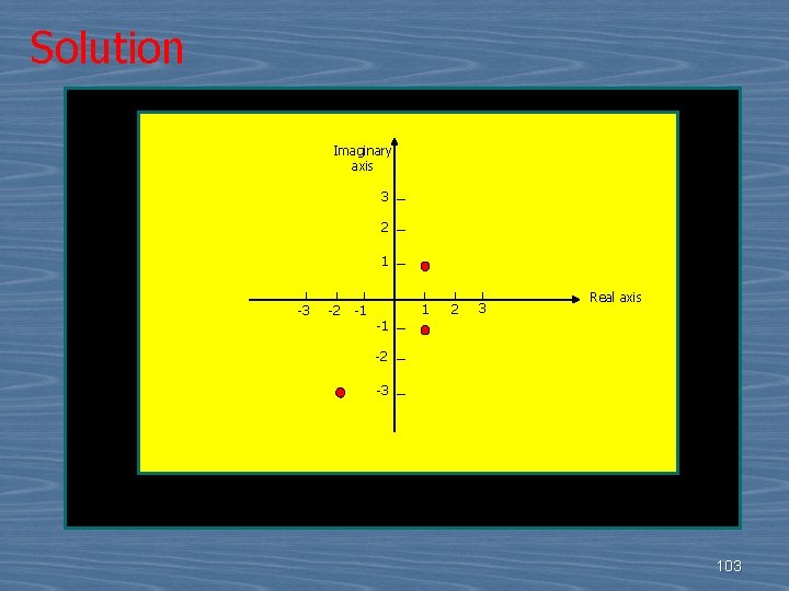
The representation of complex numbers by points in a plane is called an Argand diagram Example 1 Represent , and on an Argand diagram 102

Solution Imaginary axis 3 2 1 -3 -2 -1 1 2 3 Real axis -1 -2 -3 103

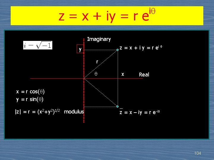
z = x + iy = r e i Imaginary z = x + i y = r ei y r x Real x = r cos( ) y = r sin( ) |z| = r = (x 2+y 2)1/2 modulus _ z = x – iy = r e-i 104

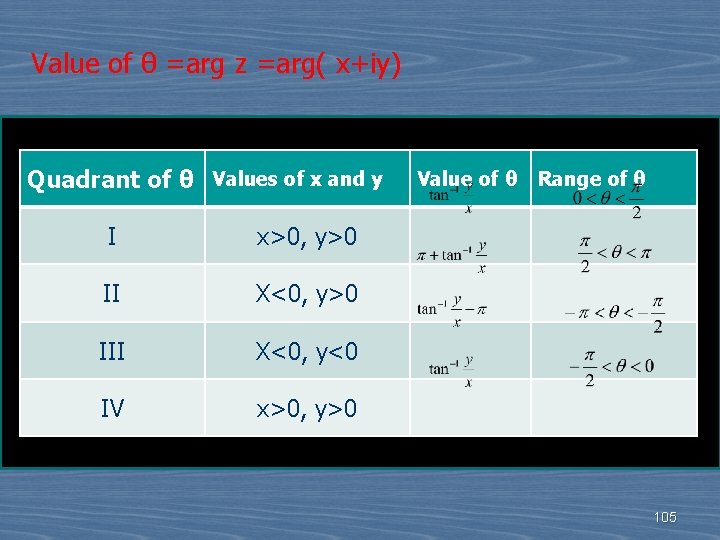
Value of θ =arg z =arg( x+iy) Quadrant of θ Values of x and y I x>0, y>0 II X<0, y>0 III X<0, y<0 IV x>0, y>0 Value of θ Range of θ 105

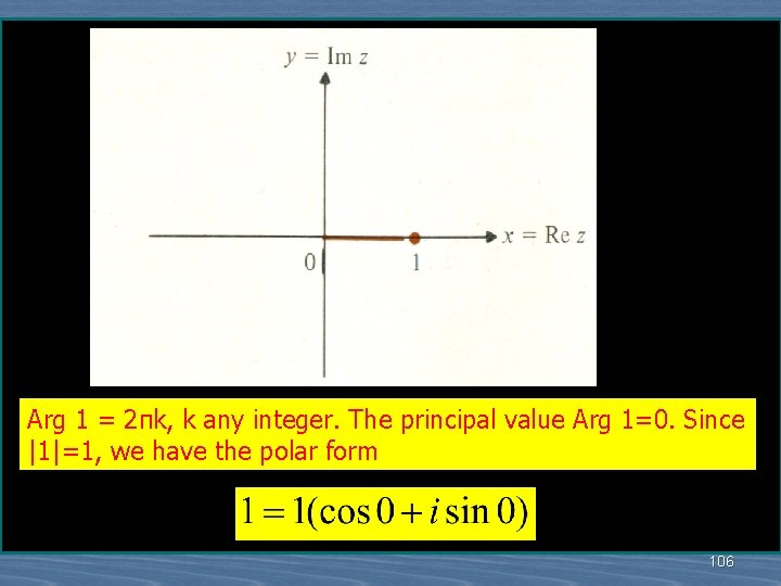
Arg 1 = 2πk, k any integer. The principal value Arg 1=0. Since |1|=1, we have the polar form 106

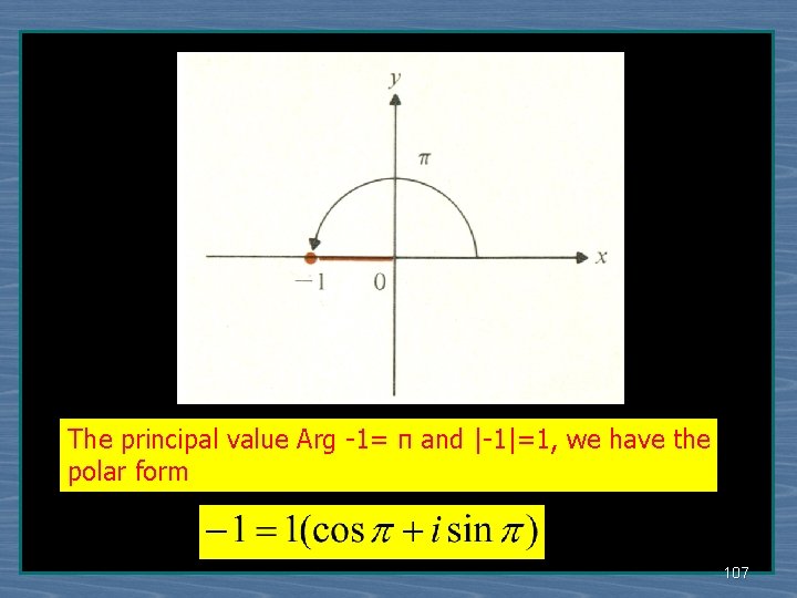
The principal value Arg -1= π and |-1|=1, we have the polar form 107

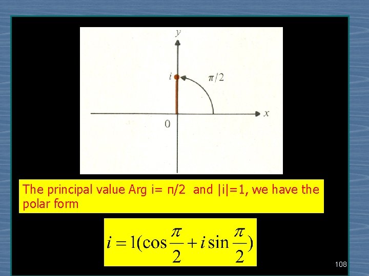
The principal value Arg i= π/2 and |i|=1, we have the polar form 108

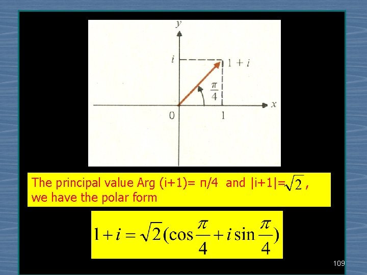
The principal value Arg (i+1)= π/4 and |i+1|= , we have the polar form 109

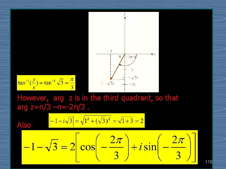
However, arg z is in the third quadrant, so that arg z=π/3 –π=-2π/3. Also 110

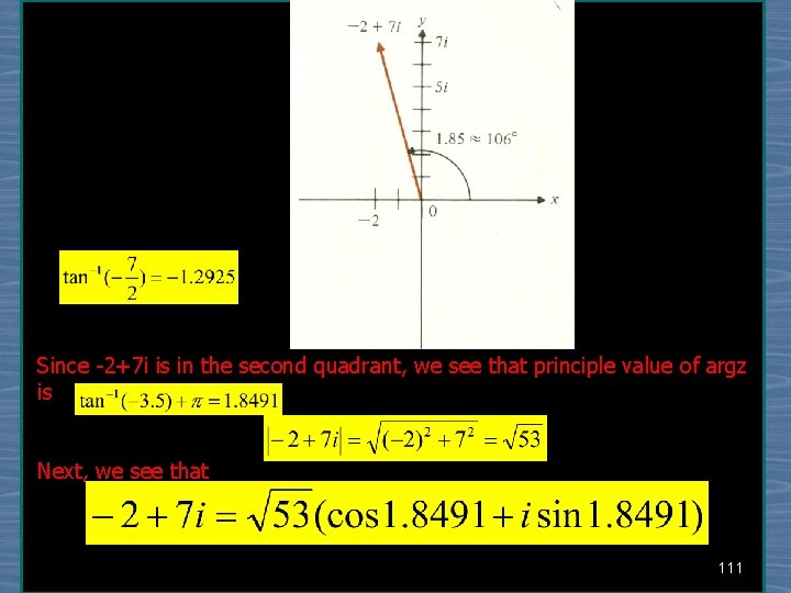
Since -2+7 i is in the second quadrant, we see that principle value of argz is Next, we see that 111

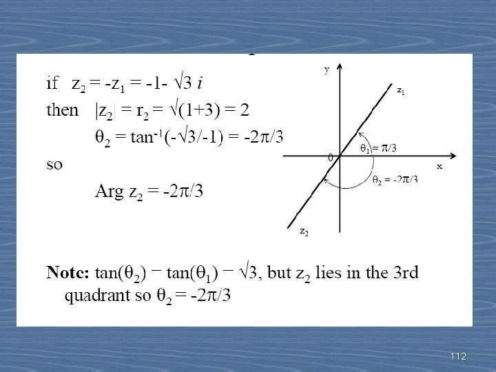
112

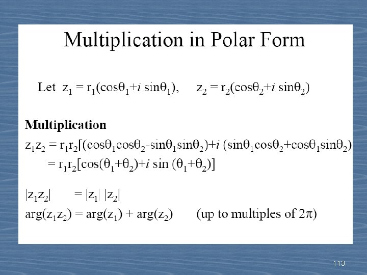
113

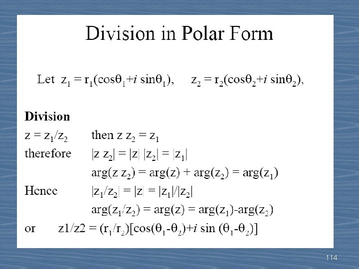
114

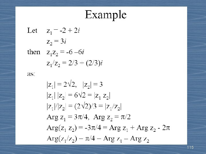
115

Don’t Forget your Homework 116

Questions? Discussion? Suggestions ? 117

118