DREAM IDEA PLAN IMPLEMENTATION ModernControlLecture Present to Amirkabir

DREAM IDEA PLAN IMPLEMENTATION
 & Semnan University Dr. Kourosh")
Modern-Control-Lecture Present to: Amirkabir University of Technology (Tehran Polytechnic) & Semnan University Dr. Kourosh Kiani Email: kkiani 2004@yahoo. com Email: Kourosh. kiani@aut. ac. ir Web: aut. ac. com 2

Lecture 7

Minimal realization & Stability of Linear Systems
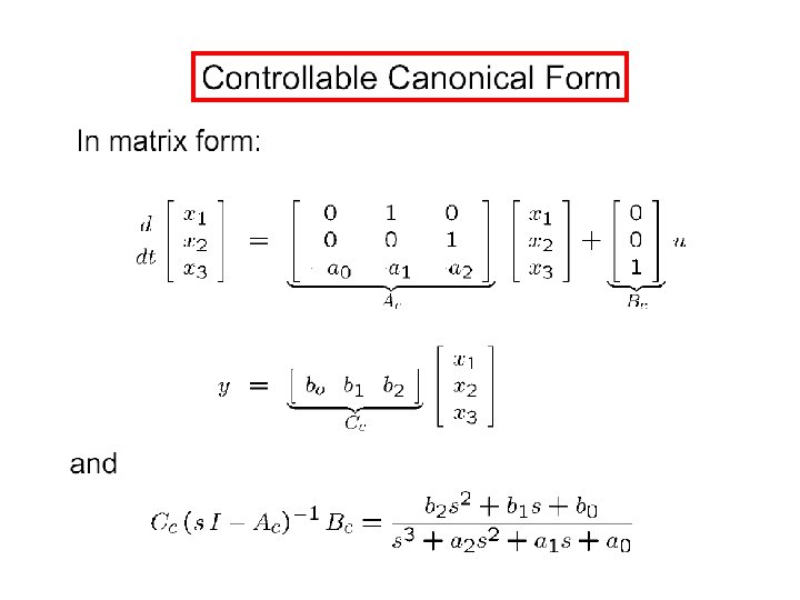

Observable Canonical Form

These realizations are guaranteed to be either controllable, or observable, but not necessarily both. They are both controllable and observable at the same time if and only if the transfer function is irreducible. Irreducible means that numerator and denominator have no common factor An example of a reducible transfer function is. If we “blindly apply the above formula for control canonical form, we get a realization of dimension 2. If we cancel (s+1) first, then we only get a realization of dimension 1. The former has dynamics that, although controllable by construction, they are not observable.

Example: Consider the transfer function Clearly, this can be reduced to a lower order one, since If we proceed to construct a controllable realization based on (1), this will not be observable, e. g. , note that for: The observability matrix is Which is of rank 1.
, this will")
Similarly, If we proceed to construct a observable realization based on (1), this will not be controllable, e. g. , The controllability matrix is Which is of rank 1.

It is interesting to note that the two, i. e. , the control canonical form and the observer canonical form relate via

Decomposition of Systems Lemma 1: Consider the n-dimensional, uncontrollable time-invariant system (A, B, C, D) where rank Rc=v<n. The system can be transformed into the following form by a nonsingular transformation z =Px; Where linearly independent columns of the controllability matrix and the last (n-v) columns are chosen to make Q nonsingular. In the transformation z=Px we are actually using the columns of as new basis vectors of the state space.

Example: The state equation is not controllable The first two columns of Q are the first two linearly independent columns of Rc; the last column of Q is chosen arbitrarily to make Q nonsingular.

Decomposition of Systems Lemma 1: Consider the n-dimensional, unobservable time-invariant system (A, B, C, D) where rank Ro= v<n. The system can be transformed into the following form by a nonsingular transformation z =Px; Where linearly independent rows of the observability matrix and the last (n-v) rows are chosen to make P nonsingular.

Example: The state equation is not observable The first two rows of P are the first two linearly independent rows of Rc; the last row of P is chosen arbitrarily to make P nonsingular. The controllability matrix of this subsystem has rank 1<2, the observable subsystem is not controllable.

It is to be noted from these examples that the decomposition of Lemma 1 or Lemma 2 does not guarantee that the acquired subsystem is both controllable and observable. A general result concerning decomposition into a system which contains a controllable and observable subsystem is obtained by combining these two Lemmas. This result, due to Kalman, is called canonical decomposition theorem and may be stated as follows. Theorem 1: Consider the linear time-invariant system (A, B, C, D). There exists a nonsingular transformation z=Px such that is both controllable and observable is controllable and unobservable is uncontrollable and unobservable
 of a system, its transfer-function matrix")
Given the state-space representation (A, B, C, D) of a system, its transfer-function matrix is uniquely determined as: However, the converse is not true, that is , given the transfer function G(s) of a system, there exists many state space representations of different orders (dimensions) that realize the same G(s). A realization (A, B, C, D) of dimension n of the transfer function matrix G(s) is said to be minimal or irreducible if no realization of order less than n exists for G(s). Note that the minimal realization is not itself unique in the sense that there exists many realizations (A 1, B 1, C 1, D 1) , (A 2, B 2, C 2, D 2), …. . Such that dim(A 1) = dim(A 2)=……. . which realize the same G(s)

is both controllable and observable is controllable and unobservable is uncontrollable and unobservable Theorem 2: A realization (A, B, C, D) of the transfer function matrix G(s) is minimal, if and only if it is both controllable and observable.

Example: The first two columns of Q are the first two linearly independent columns of Rc; the two last columns of Q is chosen arbitrarily to make Q nonsingular.

The controllable and observable subsystem is

The transfer function of this subsystem is Now consider the transfer function of the overall system: Thus the transfer-function of the overall system and of the controllable and observable subsystem are identical. This is due to the cancellations of uncontrollable modes s=0. 7±j 3. 0

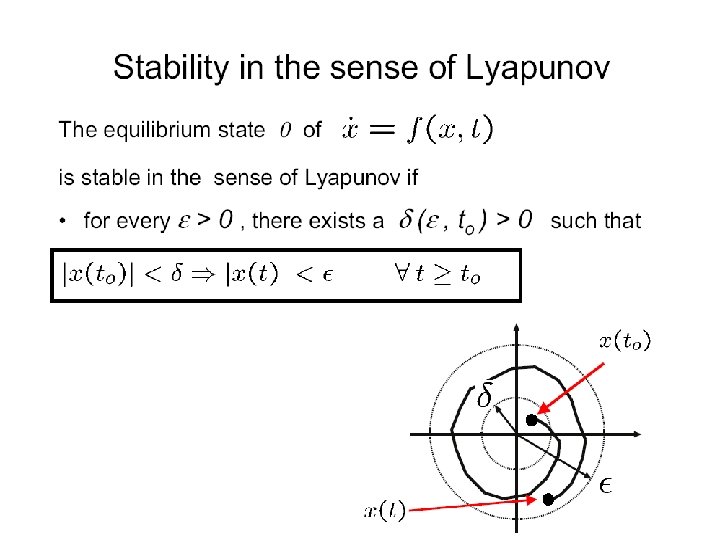
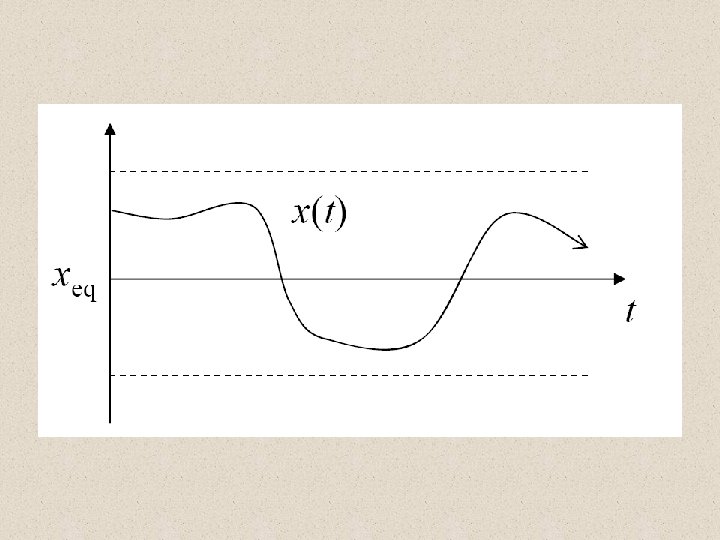
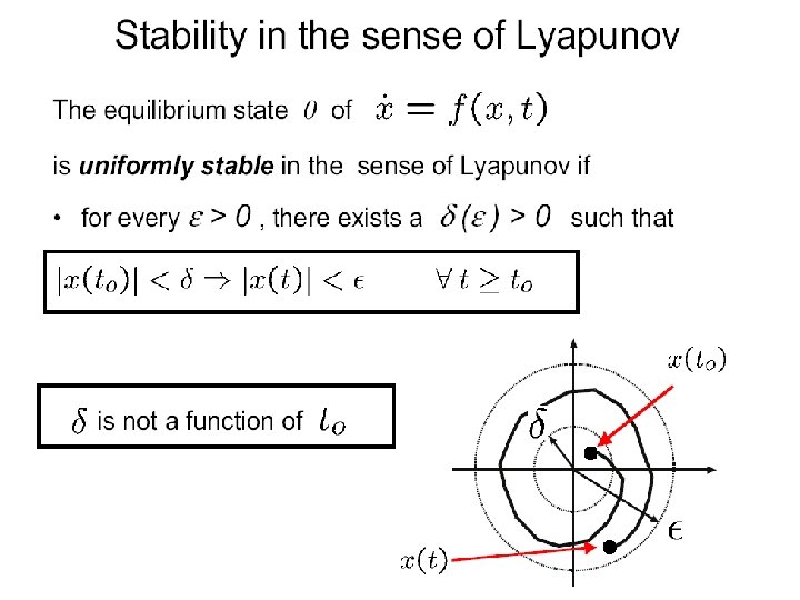
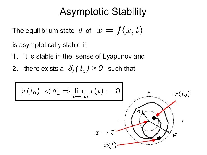
Stability of Linear Systems

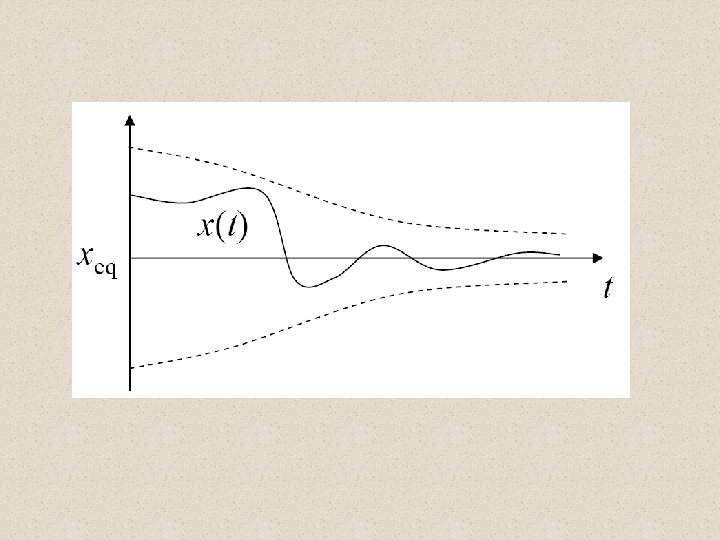
Basic Notion of Stability An important property of dynamic systems Stability. . . An “insensitivity” to small perturbations Perturbations are modeling errors of system, environment, noise F=0. OK

Basic Notions of Stability An important property of dynamic systems Stability. . . An “insensitivity” to small perturbations Perturbations are modeling errors of system, environment F=0. OK

Basic Notions of Stability An important property of dynamic systems Stability. . . An “insensitivity” to small perturbations Perturbations are modeling errors of system, environment F=0. OK

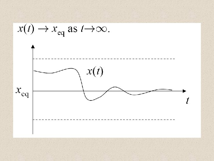
Stability n n If a system is unstable, it will degenerate when a signal, no matter how small, is applied. Stability is a basic requirement for all systems. The response of linear systems can always be decomposed into zero-state response and zeroinput response. It is customary to study the stabilities of these two components separately, i. e. Zero-state response BIBO stability Zero-input response Marginal Stability (MS) Asymptotic Stability (AS)

Input-Output Stability of LTI Systems n Consider the SISO LTI system described by where g(t) is the impulse response. n Recall for the LTI system to have an input-output description, it must be initially relaxed at t = 0 n An input u(t) is said to be bounded if there exists a constant Umax such that |u(t)| £ Umax < ¥ for all t ³ 0
")
Theorem – A SISO LTI system is BIBO stable iff its impulse response g(t) is absolutely integrable in [0, ), or for some constant M. Proof: n Show if g(t) is absolutely integrable, then every bounded input excites a bounded output. Let u(t) be an arbitrary input such that |u(t)| £ Umax< ¥ for all t ³ 0. Then
 is bounded. BIBO Stable")
Cauchy-Schwarz Norm inequality Thus, the output y(t) is bounded. BIBO Stable
 is BIBO stable")
Theorem n A SISO LTI system with proper transfer function G(s) is BIBO stable iff every pole of G(s) has a negative real part. i. e. , every pole pi lies inside the left-half s-plane
![MIMO Systems Theorem A MIMO LTI system with impulse response matrix G(t) = [gij(t)]](http://slidetodoc.com/presentation_image_h/19da91e8155324fbcd4bd852487b3c8f/image-30.jpg "MIMO Systems Theorem A MIMO LTI system with impulse response matrix G(t) = [gij(t)]")
MIMO Systems Theorem A MIMO LTI system with impulse response matrix G(t) = [gij(t)] is BIBO stable iff every gij(t) is absolutely integrable in [0, ), or for some constant Mij

Theorem – A MIMO LTI system with proper transfer function matrix is BIBO stable iff every pole of every Gij(s) has a negative real part.
 BIBO stable")
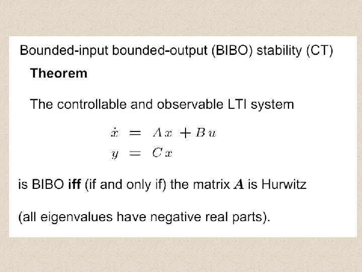
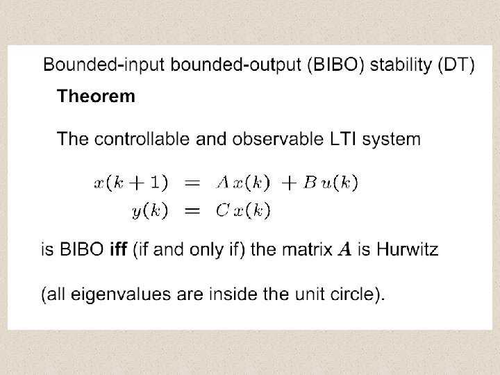
n Now, let us consider n zero-state response, is BIBO stable eig(A) BIBO stable

Questions? Discussion? Suggestions ?

- Slides: 48