DREAM IDEA PLAN IMPLEMENTATION Genetic algorithms Present to

DREAM IDEA PLAN IMPLEMENTATION

Genetic algorithms Present to: Amirkabir University of Technology (Tehran Polytechnic) & Semnan University Dr. Kourosh Kiani Email: kkiani 2004@yahoo. com Email: Kourosh. kiani@aut. ac. ir Web: aut. ac. com

Charles Darwin 1809 - 1882 "A man who dares to waste an hour of life has not discovered the value of life"

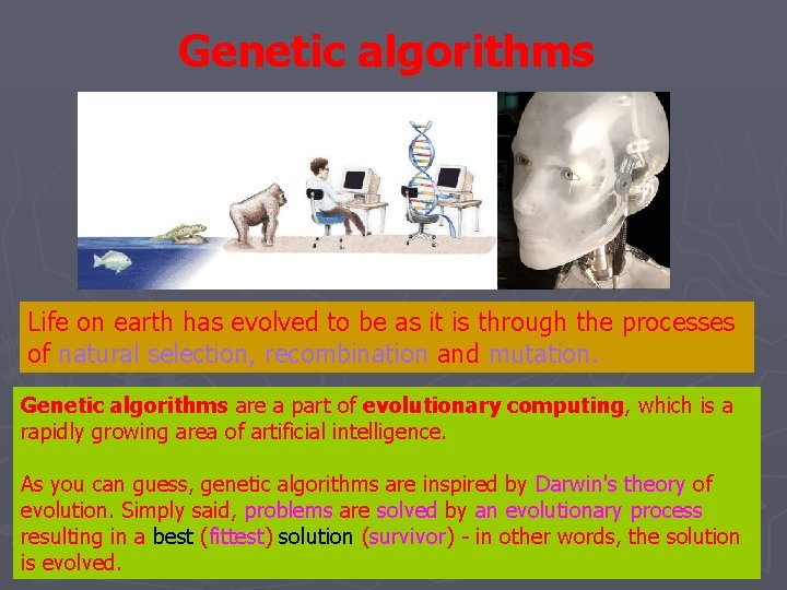
Genetic algorithms Life on earth has evolved to be as it is through the processes of natural selection, recombination and mutation. Genetic algorithms are a part of evolutionary computing, which is a rapidly growing area of artificial intelligence. As you can guess, genetic algorithms are inspired by Darwin's theory of evolution. Simply said, problems are solved by an evolutionary process resulting in a best (fittest) solution (survivor) - in other words, the solution is evolved.

History Evolutionary computing was introduced in the 1960 s by I. Rechenberg in his work "Evolution strategies" (Evolutions strategy in original). His idea was then developed by other researchers. Genetic Algorithms (GAs) were invented by John Holland developed by him and his students and colleagues. This lead to Holland's book " Adaption in Natural and Artificial Systems" published in 1975. In 1992 John Koza has used genetic algorithm to evolve programs to perform certain tasks. He called his method "genetic programming" (GP). LISP programs were used, because programs in this language can expressed in the form of a "parse tree", which is the object the GA works on.

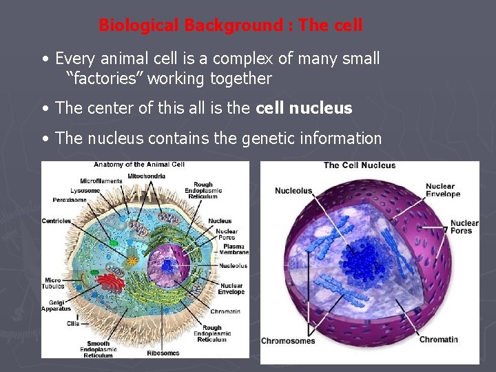
Biological Background : The cell • Every animal cell is a complex of many small “factories” working together • The center of this all is the cell nucleus • The nucleus contains the genetic information

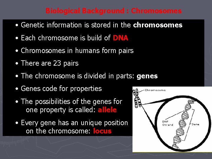
Biological Background : Chromosomes • Genetic information is stored in the chromosomes • Each chromosome is build of DNA • Chromosomes in humans form pairs • There are 23 pairs • The chromosome is divided in parts: genes • Genes code for properties • The possibilities of the genes for one property is called: allele • Every gene has an unique position on the chromosome: locus

Genetic algorithms Every organism has a set of rules, describing how that organism is built up from the tiny building blocks of life. These rules are encoded in the genes of an organism, which in turn are connected together into long strings called chromosomes. Each gene represents a specific characteristic of the organism, like eye color or hair color, and has several different settings. For example, the settings for a hair color gene may be blonde or black. These genes and their settings are usually referred to as an organism's genotype. The physical expression of the genotype - the organism itself - is called the phenotype. When two organisms mate they share their genes. The resultant offspring may end up having half the genes from one parent and half from the other. This process is called recombination. Very occasionally a gene may be mutated. Normally this mutated gene will not affect the development of the phenotype but very occasionally it will be expressed in the organism as a completely new characteristic.

What Are Genetic Algorithms? ► A way to employ evolution in the computer ► Search and optimization technique based on variation and selection

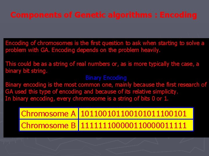
Components of Genetic algorithms : Encoding of chromosomes is the first question to ask when starting to solve a problem with GA. Encoding depends on the problem heavily. This could be as a string of real numbers or, as is more typically the case, a binary bit string. Binary Encoding Binary encoding is the most common one, mainly because the first research of GA used this type of encoding and because of its relative simplicity. In binary encoding, every chromosome is a string of bits 0 or 1. Chromosome A 101100101011100101 Chromosome B 11111110000011111

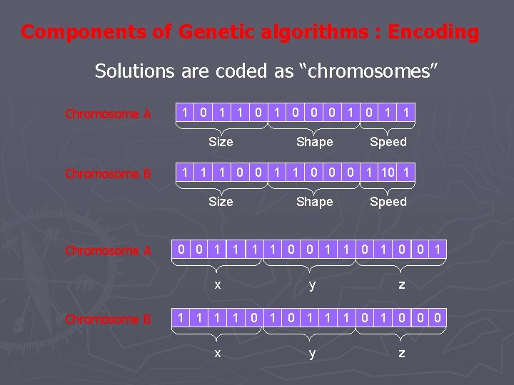
Components of Genetic algorithms : Encoding Solutions are coded as “chromosomes” Chromosome A 1 0 1 0 0 0 1 1 Size Chromosome B Shape Speed 0 0 1 1 0 0 1 x Chromosome B Speed 1 1 1 0 0 0 1 10 1 Size Chromosome A Shape y z 1 1 0 1 1 1 0 0 0 x y z

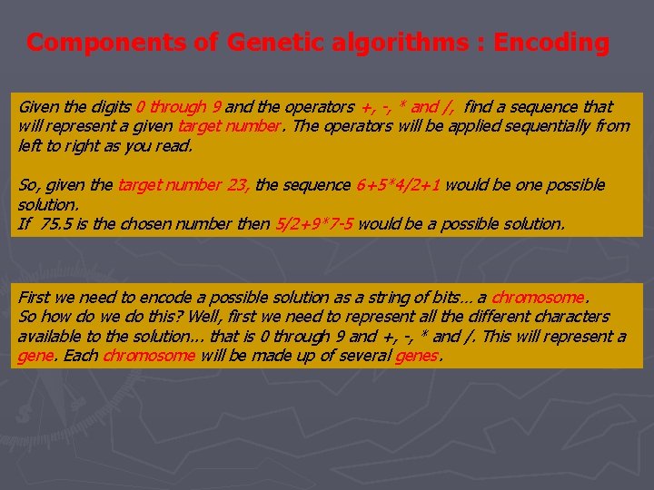
Components of Genetic algorithms : Encoding Given the digits 0 through 9 and the operators +, -, * and /, find a sequence that will represent a given target number. The operators will be applied sequentially from left to right as you read. So, given the target number 23, the sequence 6+5*4/2+1 would be one possible solution. If 75. 5 is the chosen number then 5/2+9*7 -5 would be a possible solution. First we need to encode a possible solution as a string of bits… a chromosome. So how do we do this? Well, first we need to represent all the different characters available to the solution. . . that is 0 through 9 and +, -, * and /. This will represent a gene. Each chromosome will be made up of several genes.

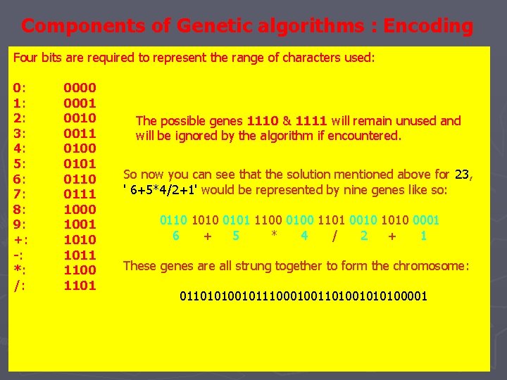
Components of Genetic algorithms : Encoding Four bits are required to represent the range of characters used: 0: 0000 1: 0001 2: 0010 The possible genes 1110 & 1111 will remain unused and 3: 0011 will be ignored by the algorithm if encountered. 4: 0100 5: 0101 So now you can see that the solution mentioned above for 23, 6: 0110 ' 6+5*4/2+1' would be represented by nine genes like so: 7: 0111 8: 1000 0110 1010 0101 1100 0100 1101 0010 1010 0001 9: 1001 6 + 5 * 4 / 2 + 1 +: 1010 -: 1011 These genes are all strung together to form the chromosome: *: 1100 /: 1101 011010100101110001001101001010100001

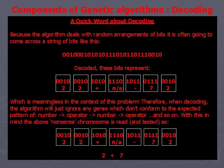
Components of Genetic algorithms : Decoding A Quick Word about Decoding Because the algorithm deals with random arrangements of bits it is often going to come across a string of bits like this: 001010101101110010 Decoded, these bits represent: 0010 1010 1110 1011 0111 0010 2 2 + n/a - 7 2 Which is meaningless in the context of this problem! Therefore, when decoding, the algorithm will just ignore any genes which don’t conform to the expected pattern of: number -> operator -> number -> operator …and so on. With this in mind the above ‘nonsense’ chromosome is read (and tested) as: 0010 1010 1110 1011 0111 0010 2 2 + n/a - 7 2 2 + 7

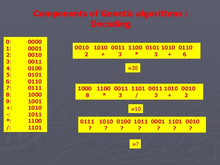
Components of Genetic algorithms : Decoding 0: 1: 2: 3: 4: 5: 6: 7: 8: 9: +: -: *: /: 0000 0001 0010 0011 0100 0101 0110 0111 1000 1001 1010 1011 1100 1101 0010 1010 0011 1100 0101 1010 0110 2 + 3 * 5 + 6 =30 1000 1100 0011 1101 0011 1010 0010 8 * 3 / 3 + 2 =10 0111 1010 0100 1011 0001 1101 0010 ? ? =?

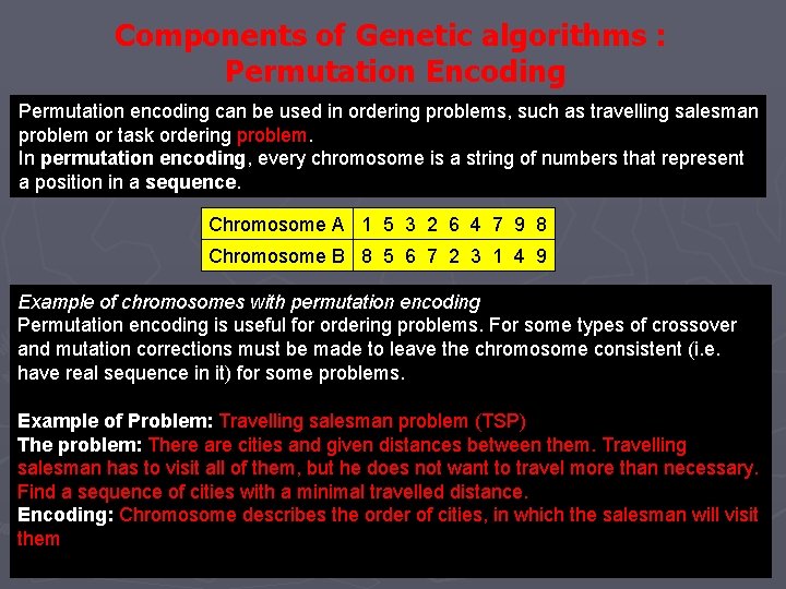
Components of Genetic algorithms : Permutation Encoding Permutation encoding can be used in ordering problems, such as travelling salesman problem or task ordering problem. In permutation encoding, every chromosome is a string of numbers that represent a position in a sequence. Chromosome A 1 5 3 2 6 4 7 9 8 Chromosome B 8 5 6 7 2 3 1 4 9 Example of chromosomes with permutation encoding Permutation encoding is useful for ordering problems. For some types of crossover and mutation corrections must be made to leave the chromosome consistent (i. e. have real sequence in it) for some problems. Example of Problem: Travelling salesman problem (TSP) The problem: There are cities and given distances between them. Travelling salesman has to visit all of them, but he does not want to travel more than necessary. Find a sequence of cities with a minimal travelled distance. Encoding: Chromosome describes the order of cities, in which the salesman will visit them

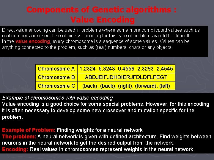
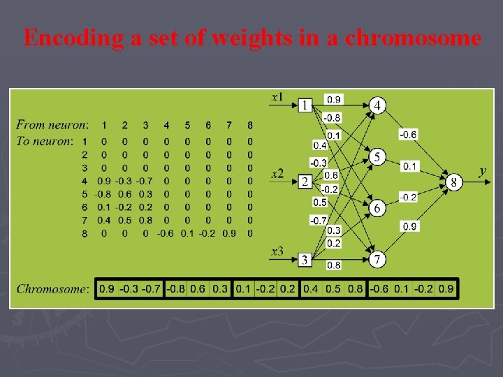
Components of Genetic algorithms : Value Encoding Direct value encoding can be used in problems where some more complicated values such as real numbers are used. Use of binary encoding for this type of problems would be difficult. In the value encoding, every chromosome is a sequence of some values. Values can be anything connected to the problem, such as (real) numbers, chars or any objects. Chromosome A 1. 2324 5. 3243 0. 4556 2. 3293 2. 4545 Chromosome B ABDJEIFJDHDIERJFDLDFLFEGT Chromosome C (back), (right), (forward), (left) Example of chromosomes with value encoding Value encoding is a good choice for some special problems. However, for this encoding it is often necessary to develop some new crossover and mutation specific for the problem. Example of Problem: Finding weights for a neural network The problem: A neural network is given with defined architecture. Find weights between neurons in the neural network to get the desired output from the network. Encoding: Real values in chromosomes represent weights in the neural network.

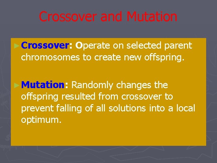
Crossover and Mutation ► Crossover: Operate on selected parent chromosomes to create new offspring. ► Mutation: Randomly changes the offspring resulted from crossover to prevent falling of all solutions into a local optimum.

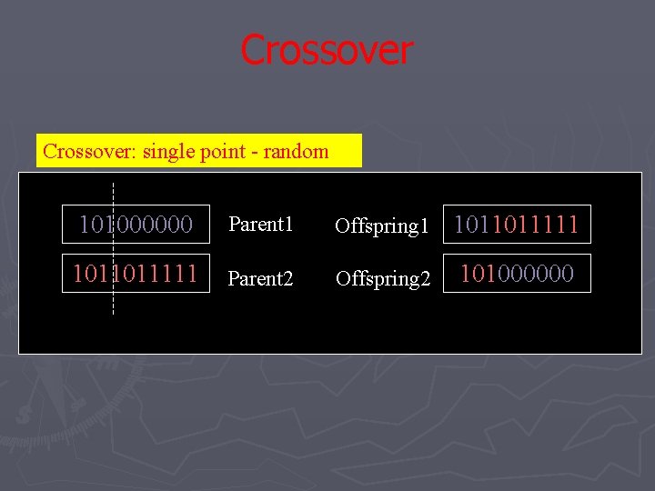
Crossover: single point - random 101000000 Parent 1 Offspring 1 1011011111 Parent 2 Offspring 2 101000000

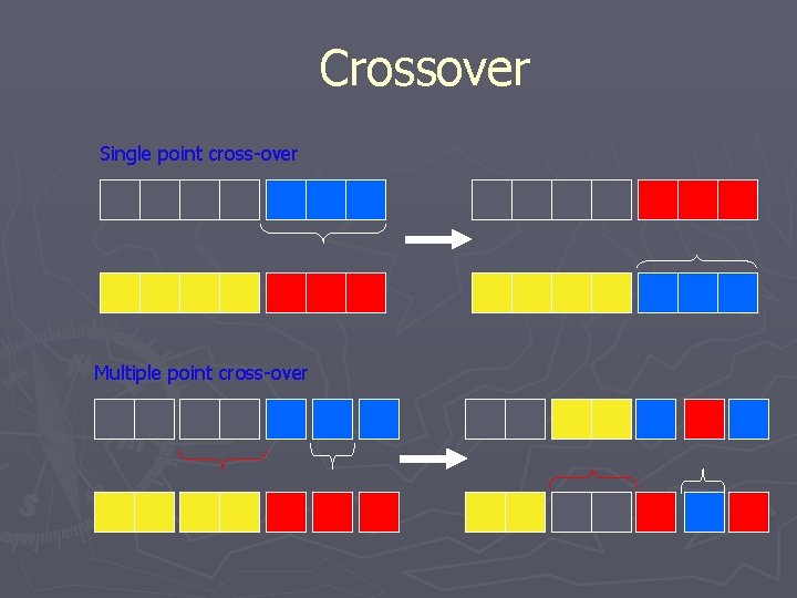
Crossover Single point cross-over Multiple point cross-over

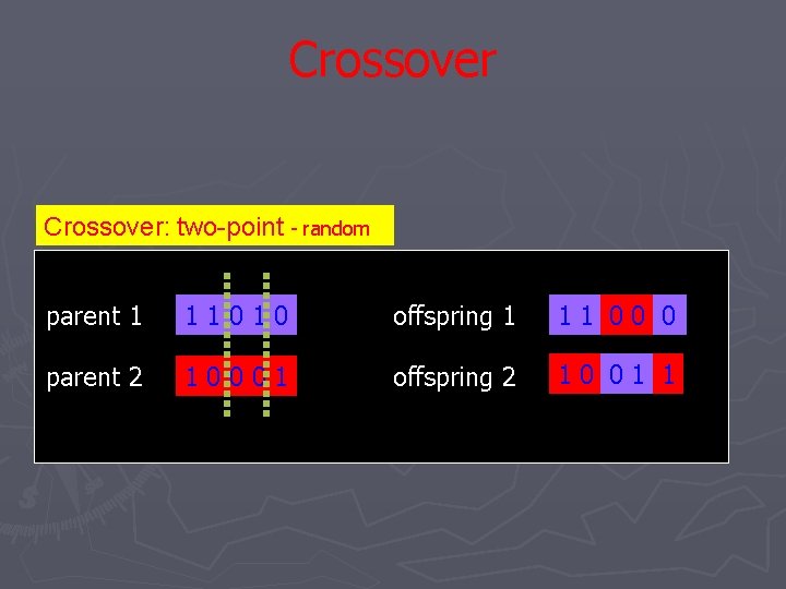
Crossover: two-point - random parent 1 1 1 0 offspring 1 1 1 0 0 0 parent 2 1 0 0 0 1 offspring 2 1 0 0 1 1

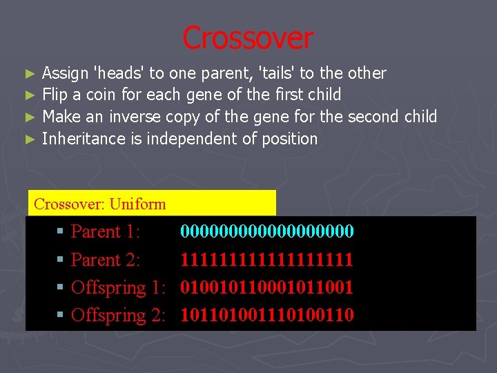
Crossover Assign 'heads' to one parent, 'tails' to the other ► Flip a coin for each gene of the first child ► Make an inverse copy of the gene for the second child ► Inheritance is independent of position ► Crossover: Uniform § § Parent 1: Parent 2: Offspring 1: Offspring 2: 000000000 111111111 01001011001 10110100110

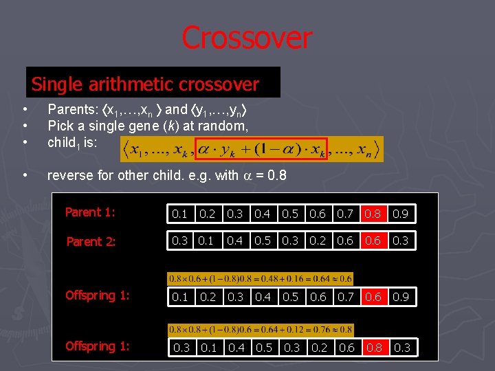
Crossover Single arithmetic crossover • • • Parents: x 1, …, xn and y 1, …, yn Pick a single gene (k) at random, child 1 is: • reverse for other child. e. g. with = 0. 8 Parent 1: 0. 1 0. 2 0. 3 0. 4 0. 5 0. 6 0. 7 0. 8 0. 9 Parent 2: 0. 3 0. 1 0. 4 0. 5 0. 3 0. 2 0. 6 0. 3 Offspring 1: 0. 1 0. 2 0. 3 0. 4 0. 5 0. 6 0. 7 0. 6 0. 9 Offspring 1: 0. 3 0. 1 0. 4 0. 5 0. 3 0. 2 0. 6 0. 8 0. 3

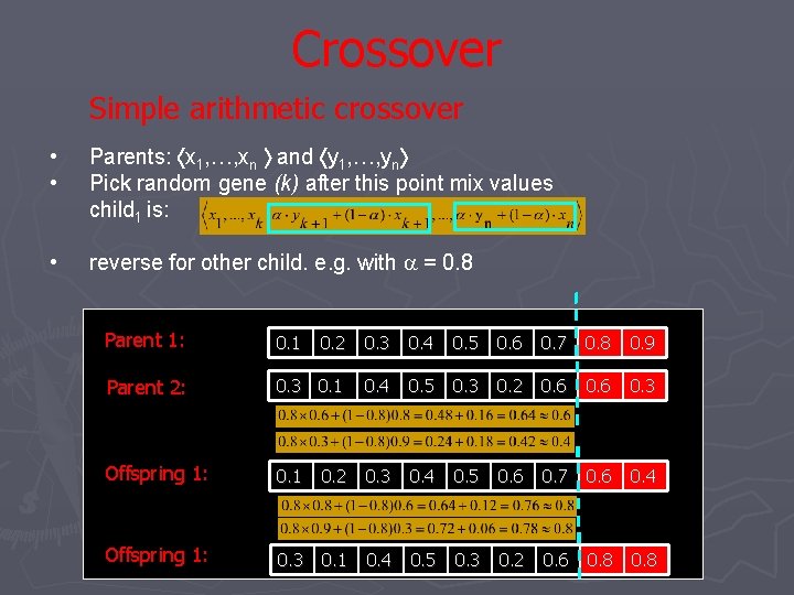
Crossover Simple arithmetic crossover • • Parents: x 1, …, xn and y 1, …, yn Pick random gene (k) after this point mix values child 1 is: • reverse for other child. e. g. with = 0. 8 Parent 1: 0. 1 0. 2 0. 3 0. 4 0. 5 0. 6 0. 7 0. 8 0. 9 Parent 2: 0. 3 0. 1 0. 4 0. 5 0. 3 0. 2 0. 6 0. 3 Offspring 1: 0. 1 0. 2 0. 3 0. 4 0. 5 0. 6 0. 7 0. 6 0. 4 Offspring 1: 0. 3 0. 1 0. 4 0. 5 0. 3 0. 2 0. 6 0. 8

Crossover None - no crossover, offspring is exact copy of parents

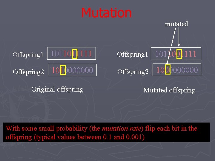
Mutation Offspring 1 1011011111 Offspring 2 1010000000 Original offspring mutated Offspring 1 1011001111 Offspring 2 100000 Mutated offspring With some small probability (the mutation rate) flip each bit in the offspring (typical values between 0. 1 and 0. 001)

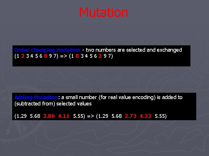
Mutation Order changing mutation - two numbers are selected and exchanged (1 2 3 4 5 6 8 9 7) => (1 8 3 4 5 6 2 9 7) Adding Mutation: a small number (for real value encoding) is added to (subtracted from) selected values (1. 29 5. 68 2. 86 4. 11 5. 55) => (1. 29 5. 68 2. 73 4. 22 5. 55)

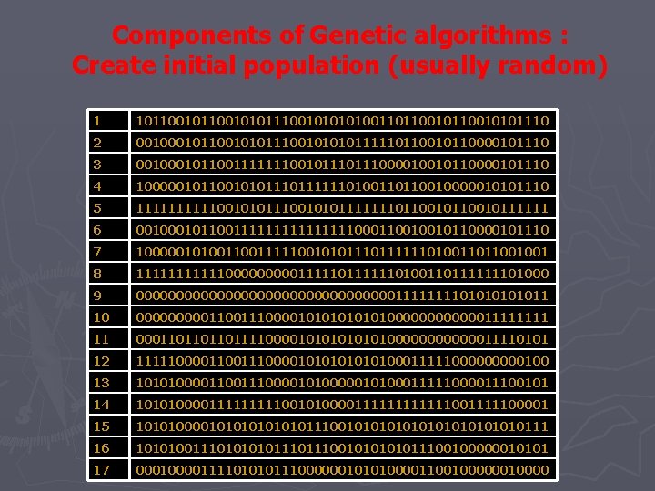
Components of Genetic algorithms : Create initial population (usually random) 1 10110010101110010100110110010101110 2 00101100101010111110110000101110 3 0010110011111110010111000010010110000101110 4 10000010110010101111110100110110010000010101110 5 1111100101011111110110010111111 6 0010110011111111000110010010110000101110 7 1000001010011111001010111111010011011001001 8 111111000001111110100110111111101000 9 000000000000000011110101011 10 0000011001110000101010000001111 11 000110111100001010100000011110101 12 1111100001110000101010001111100000100 13 101010000111000010100011111000011100101 14 10101000011111001010000111111001111100001 15 101010000101010111001010101010111 16 101010011101011100101011100100000010101 17 00010000111101010111000000101010000110010000

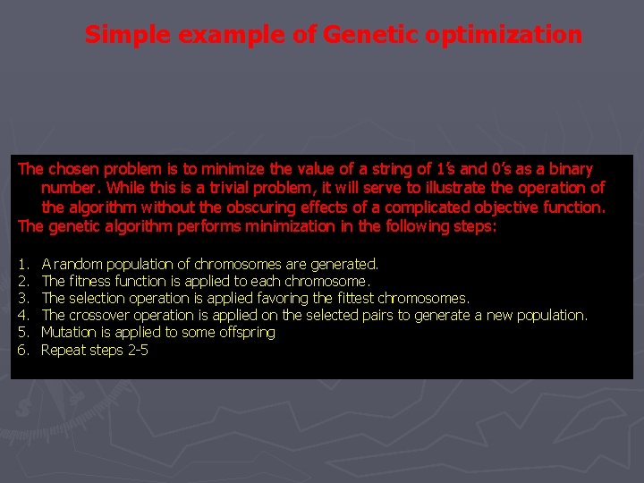
Simple example of Genetic optimization The chosen problem is to minimize the value of a string of 1’s and 0’s as a binary number. While this is a trivial problem, it will serve to illustrate the operation of the algorithm without the obscuring effects of a complicated objective function. The genetic algorithm performs minimization in the following steps: 1. 2. 3. 4. 5. 6. A random population of chromosomes are generated. The fitness function is applied to each chromosome. The selection operation is applied favoring the fittest chromosomes. The crossover operation is applied on the selected pairs to generate a new population. Mutation is applied to some offspring Repeat steps 2 -5

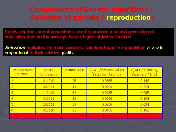
Components of Genetic algorithms : Selection of parents ( reproduction) In this step the current population is used to produce a second generation of population that, on the average, have a higher objective function. Selection replicates the most successful solutions found in a population at a rate proportional to their relative quality. J chromosome number Binary chromosome Decimal value Oj = 1/(decimal value) Objective function Fj =Oj / (Total Oj) Fraction of Total 1 011010 26 0. 0385 0. 142 2 001011 11 0. 0909 0. 334 3 110110 54 0. 0185 0. 068 4 010011 19 0. 0526 0. 194 5 100111 39 0. 0256 0. 094 6 010110 22 0. 0455 0. 168 0. 2717 1 Total

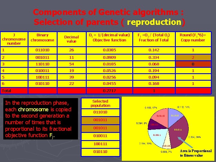
Components of Genetic algorithms : Selection of parents ( reproduction) J chromosome number Binary chromosome Decimal value Oj = 1/(decimal value) Objective function Fj =Oj / (Total Oj) Fraction of Total Round (Fj*6)= Copy number 1 011010 26 0. 0385 0. 142 1 2 001011 11 0. 0909 0. 334 2 3 110110 54 0. 0185 0. 068 0 4 010011 19 0. 0526 0. 194 1 5 100111 39 0. 0256 0. 094 1 6 010110 22 0. 0455 0. 168 1 0. 2717 1 Total In the reproduction phase, each chromosome is copied to the second generation a number of times that is proportional to its fractional objective function Fj. Selected population 011010 01011010 001011 0100111 010110 100111 001011 010011 110110 Area is Proportional to fitness value

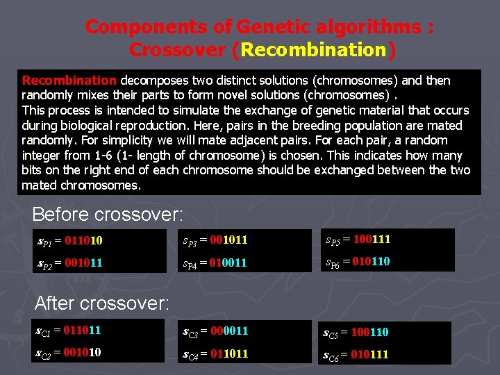
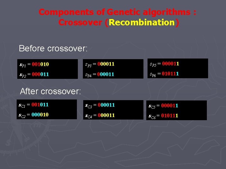
Components of Genetic algorithms : Crossover (Recombination) Recombination decomposes two distinct solutions (chromosomes) and then randomly mixes their parts to form novel solutions (chromosomes). This process is intended to simulate the exchange of genetic material that occurs during biological reproduction. Here, pairs in the breeding population are mated randomly. For simplicity we will mate adjacent pairs. For each pair, a random integer from 1 -6 (1 - length of chromosome) is chosen. This indicates how many bits on the right end of each chromosome should be exchanged between the two mated chromosomes. Before crossover: s. P 1 = 011010 s. P 3 = 001011 s. P 5 = 100111 s. P 2 = 001011 s. P 4 = 010011 s. P 6 = 010110 s. C 1 = 011011 s. C 3 = 000011 s. C 5 = 100110 s. C 2 = 001010 s. C 4 = 011011 s. C 6 = 010111 After crossover:

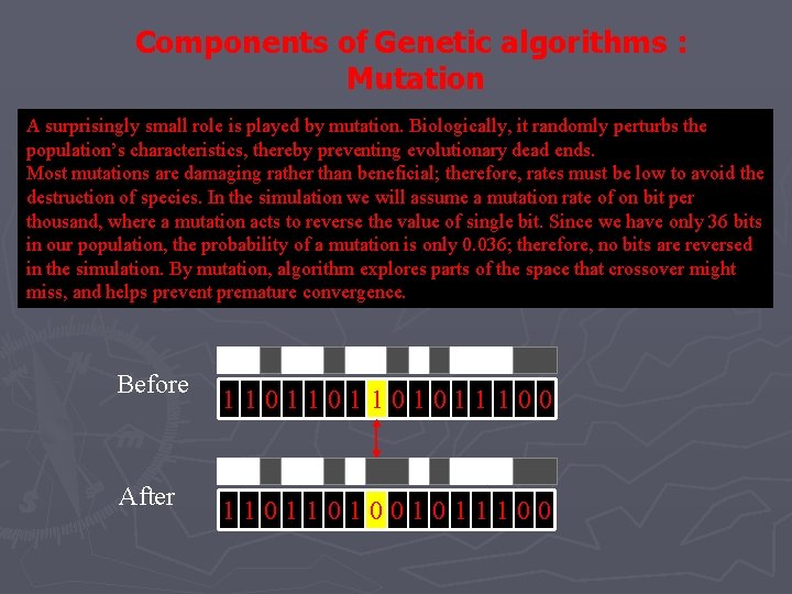
Components of Genetic algorithms : Mutation A surprisingly small role is played by mutation. Biologically, it randomly perturbs the population’s characteristics, thereby preventing evolutionary dead ends. Most mutations are damaging rather than beneficial; therefore, rates must be low to avoid the destruction of species. In the simulation we will assume a mutation rate of on bit per thousand, where a mutation acts to reverse the value of single bit. Since we have only 36 bits in our population, the probability of a mutation is only 0. 036; therefore, no bits are reversed in the simulation. By mutation, algorithm explores parts of the space that crossover might miss, and helps prevent premature convergence. Before After 1101101101011 100 1101101001011100

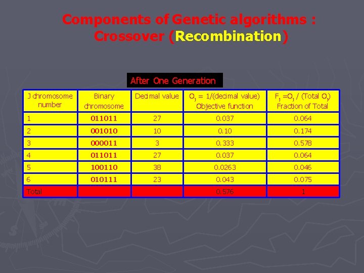
Components of Genetic algorithms : Crossover (Recombination) After One Generation J chromosome number Binary chromosome Decimal value Oj = 1/(decimal value) Objective function Fj =Oj / (Total Oj) Fraction of Total 1 011011 27 0. 037 0. 064 2 001010 10 0. 174 3 000011 3 0. 333 0. 578 4 011011 27 0. 037 0. 064 5 100110 38 0. 0263 0. 046 6 010111 23 0. 043 0. 075 0. 576 1 Total

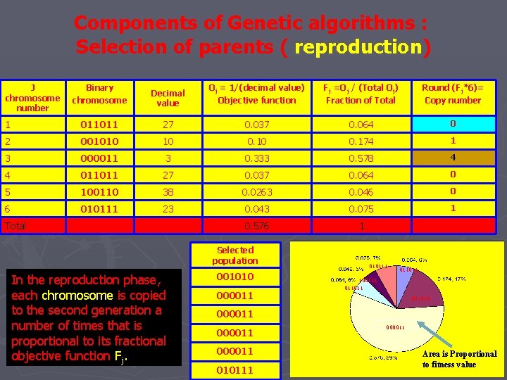
Components of Genetic algorithms : Selection of parents ( reproduction) J chromosome number Binary chromosome Decimal value Oj = 1/(decimal value) Objective function Fj =Oj / (Total Oj) Fraction of Total Round (Fj*6)= Copy number 1 011011 27 0. 037 0. 064 0 2 001010 10 0. 174 1 3 000011 3 0. 333 0. 578 4 4 011011 27 0. 037 0. 064 0 5 100110 38 0. 0263 0. 046 0 6 010111 23 0. 043 0. 075 1 0. 576 1 Total Selected population In the reproduction phase, each chromosome is copied to the second generation a number of times that is proportional to its fractional objective function Fj. 001010 000011 010111 011011 100111 011011 001010 000011 010111 000011 Area is Proportional to fitness value

Components of Genetic algorithms : Crossover (Recombination) Before crossover: s. P 1 = 001010 s. P 3 = 000011 s. P 5 = 000011 s. P 2 = 000011 s. P 4 = 000011 s. P 6 = 010111 s. C 1 = 001011 s. C 3 = 000011 s. C 5 = 000011 s. C 2 = 000010 s. C 4 = 000011 s. C 6 = 010111 After crossover:

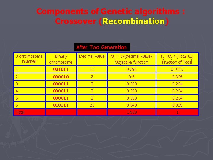
Components of Genetic algorithms : Crossover (Recombination) After Two Generation J chromosome number Binary chromosome Decimal value Oj = 1/(decimal value) Objective function Fj =Oj / (Total Oj) Fraction of Total 1 001011 11 0. 091 0. 0557 2 000010 2 0. 5 0. 306 3 000011 3 0. 333 0. 204 4 000011 3 0. 333 0. 204 5 000011 3 0. 333 0. 204 6 010111 23 0. 043 0. 026 1. 633 1 Total

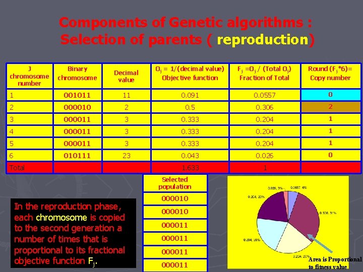
Components of Genetic algorithms : Selection of parents ( reproduction) J chromosome number Binary chromosome Decimal value Oj = 1/(decimal value) Objective function Fj =Oj / (Total Oj) Fraction of Total Round (Fj*6)= Copy number 1 001011 11 0. 091 0. 0557 0 2 000010 2 0. 5 0. 306 2 3 000011 3 0. 333 0. 204 1 4 000011 3 0. 333 0. 204 1 5 000011 3 0. 333 0. 204 1 6 010111 23 0. 043 0. 026 0 1. 633 1 Total Selected population In the reproduction phase, each chromosome is copied to the second generation a number of times that is proportional to its fractional objective function Fj. 000010 000011 Area is Proportional to fitness value

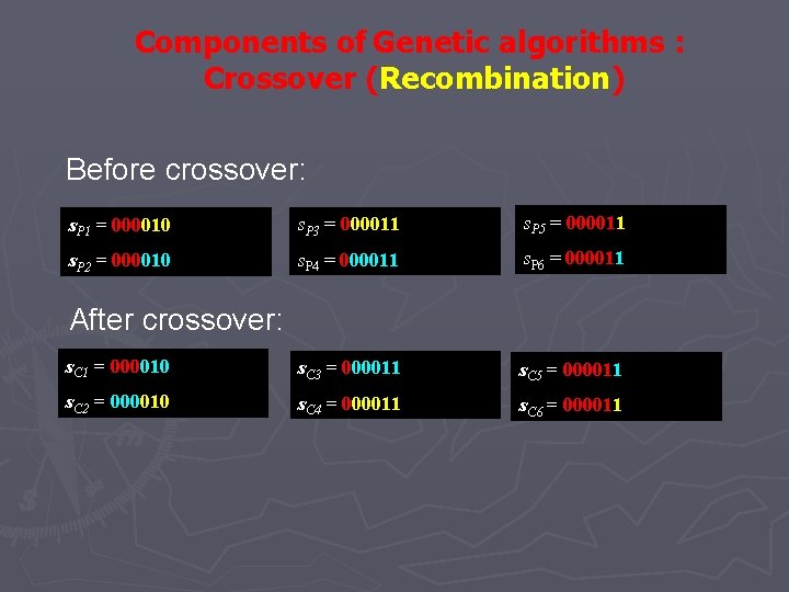
Components of Genetic algorithms : Crossover (Recombination) Before crossover: s. P 1 = 000010 s. P 3 = 000011 s. P 5 = 000011 s. P 2 = 000010 s. P 4 = 000011 s. P 6 = 000011 s. C 1 = 000010 s. C 3 = 000011 s. C 5 = 000011 s. C 2 = 000010 s. C 4 = 000011 s. C 6 = 000011 After crossover:

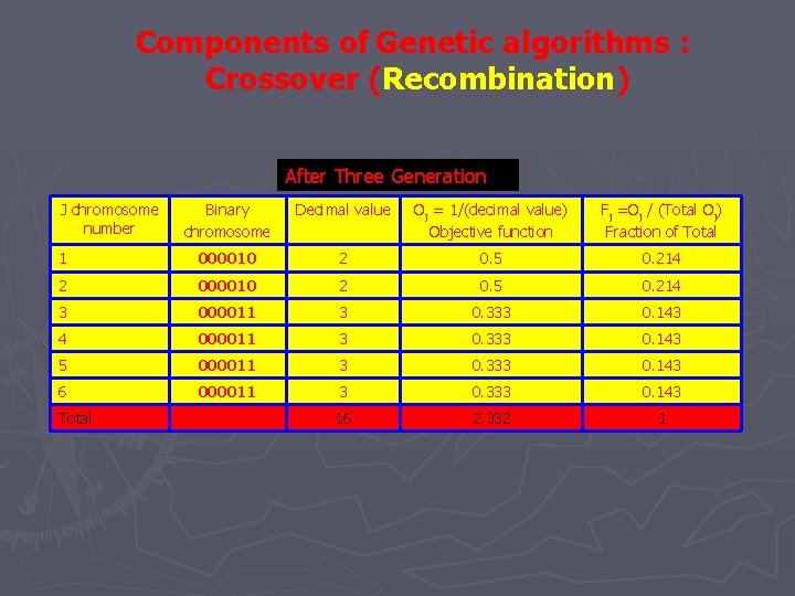
Components of Genetic algorithms : Crossover (Recombination) After Three Generation J chromosome number Binary chromosome Decimal value Oj = 1/(decimal value) Objective function Fj =Oj / (Total Oj) Fraction of Total 1 000010 2 0. 5 0. 214 2 000010 2 0. 5 0. 214 3 000011 3 0. 333 0. 143 4 000011 3 0. 333 0. 143 5 000011 3 0. 333 0. 143 6 000011 3 0. 333 0. 143 16 2. 332 1 Total

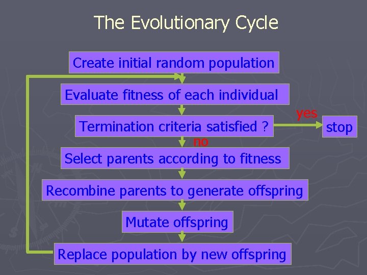
The Evolutionary Cycle Create initial random population Evaluate fitness of each individual Termination criteria satisfied ? no Select parents according to fitness yes Recombine parents to generate offspring Mutate offspring Replace population by new offspring stop

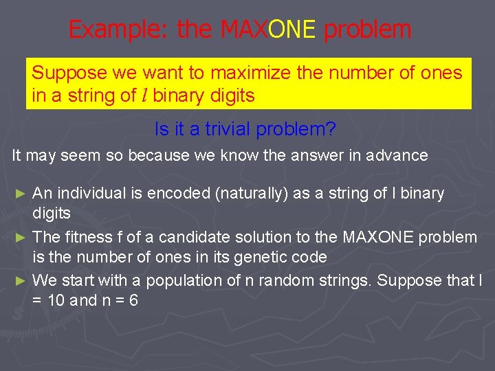
Example: the MAXONE problem Suppose we want to maximize the number of ones in a string of l binary digits Is it a trivial problem? It may seem so because we know the answer in advance An individual is encoded (naturally) as a string of l binary digits ► The fitness f of a candidate solution to the MAXONE problem is the number of ones in its genetic code ► We start with a population of n random strings. Suppose that l = 10 and n = 6 ►

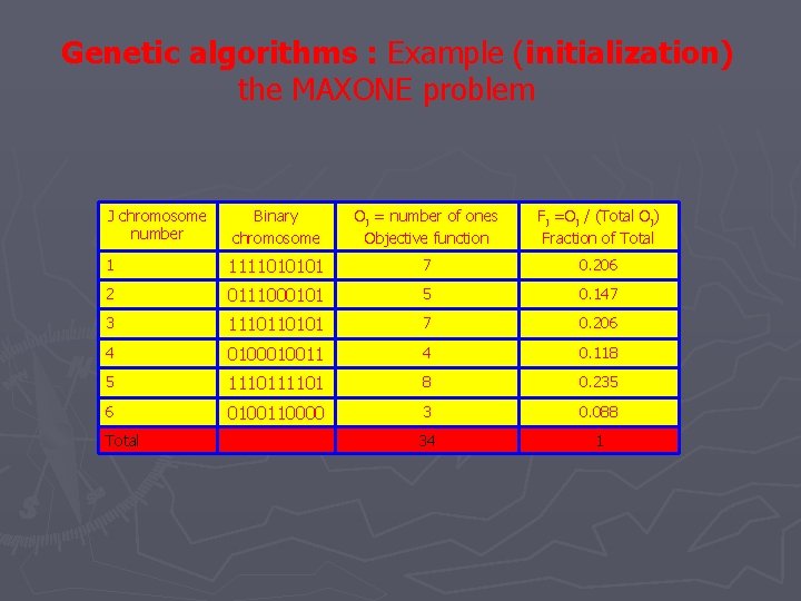
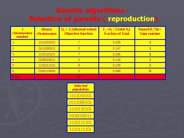
Genetic algorithms : Example (initialization) Example ( the MAXONE problem J chromosome number Binary chromosome Oj = number of ones Objective function Fj =Oj / (Total Oj) Fraction of Total 1 1111010101 7 0. 206 2 0111000101 5 0. 147 3 1110110101 7 0. 206 4 010011 4 0. 118 5 11101 8 0. 235 6 0100110000 3 0. 088 34 1 Total

Genetic algorithms : Selection of parents ( reproduction) J chromosome number Binary chromosome Oj = 1/(decimal value) Objective function Fj =Oj / (Total Oj) Fraction of Total Round (Fj*6)= Copy number 1 1111010101 7 0. 206 1 2 0111000101 5 0. 147 1 3 1110110101 7 0. 206 1 4 010011 4 0. 118 1 5 11101 8 0. 235 1 6 0100110000 3 0. 088 0 34 1 Total Selected population 1111010101 0111000101 1110110101 010011 1110111101

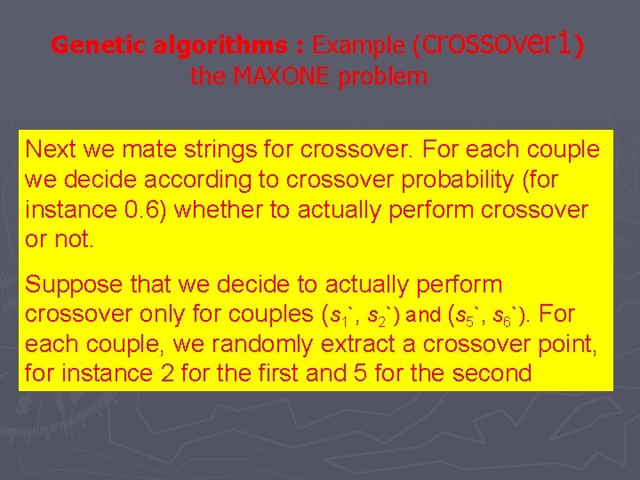
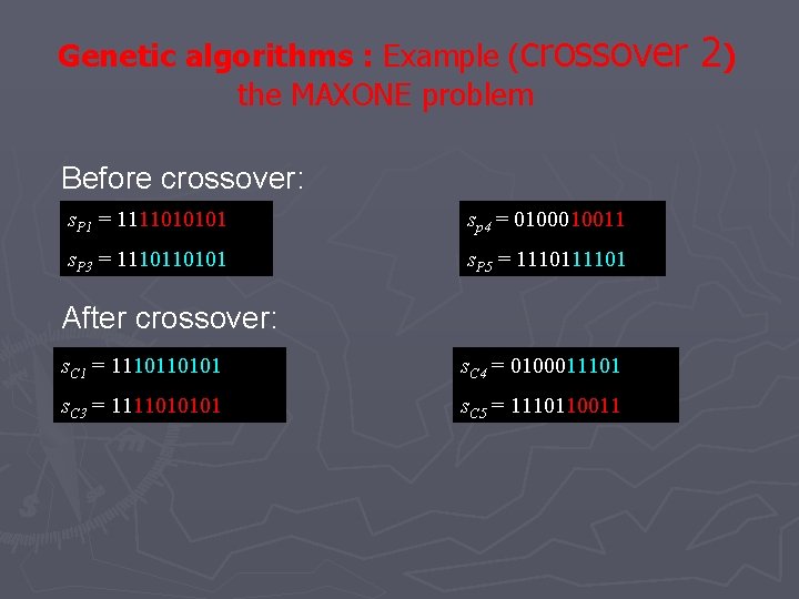
Genetic algorithms : Example (crossover 1) the MAXONE problem Next we mate strings for crossover. For each couple we decide according to crossover probability (for instance 0. 6) whether to actually perform crossover or not. Suppose that we decide to actually perform crossover only for couples (s 1`, s 2`) and (s 5`, s 6`). For each couple, we randomly extract a crossover point, for instance 2 for the first and 5 for the second

Genetic algorithms : Example (crossover 2) the MAXONE problem Before crossover: s. P 1 = 1111010101 sp 4 = 010011 s. P 3 = 1110110101 s. P 5 = 11101 After crossover: s. C 1 = 1110110101 s. C 4 = 0100011101 s. C 3 = 1111010101 s. C 5 = 1110110011

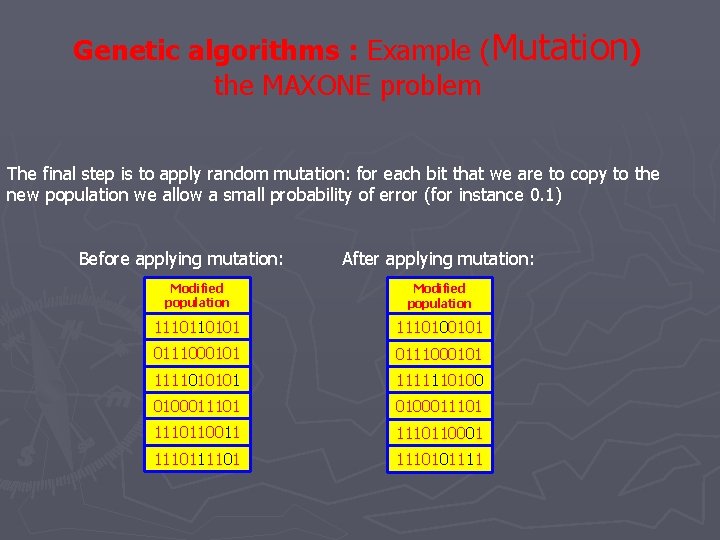
Genetic algorithms : Example (Mutation) the MAXONE problem The final step is to apply random mutation: for each bit that we are to copy to the new population we allow a small probability of error (for instance 0. 1) Before applying mutation: After applying mutation: Modified population 1110110101 1110100101 0111000101 1111010101 111111010001110110011 1110110001 1110101111

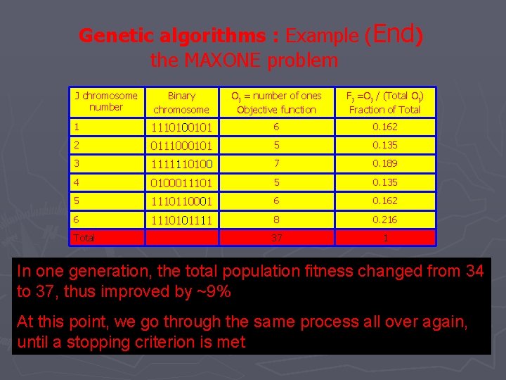
Genetic algorithms : Example (End) the MAXONE problem J chromosome number Binary chromosome Oj = number of ones Objective function Fj =Oj / (Total Oj) Fraction of Total 1 1110100101 6 0. 162 2 0111000101 5 0. 135 3 1111110100 7 0. 189 4 0100011101 5 0. 135 5 1110110001 6 0. 162 6 1110101111 8 0. 216 37 1 Total In one generation, the total population fitness changed from 34 to 37, thus improved by ~9% At this point, we go through the same process all over again, until a stopping criterion is met

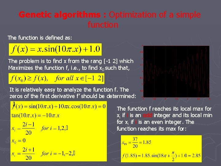
Genetic algorithms : Optimization of a simple function The function is defined as: The problem is to find x from the rang [-1 2] which Maximizes the function f, i. e. , to find x 0 such that, It is relatively easy to analyze the function f. The zeros of the first derivative f’ should be determined: The function f reaches its local max for xi if i is an odd integer and its local min for xi if i is an even integer. The function reaches its max for:

Genetic algorithms : Optimization of a simple function Assume that we wish to construct a genetic algorithm: to maximize the function f. Let discuss the major components of such a genetic algorithm in turn.

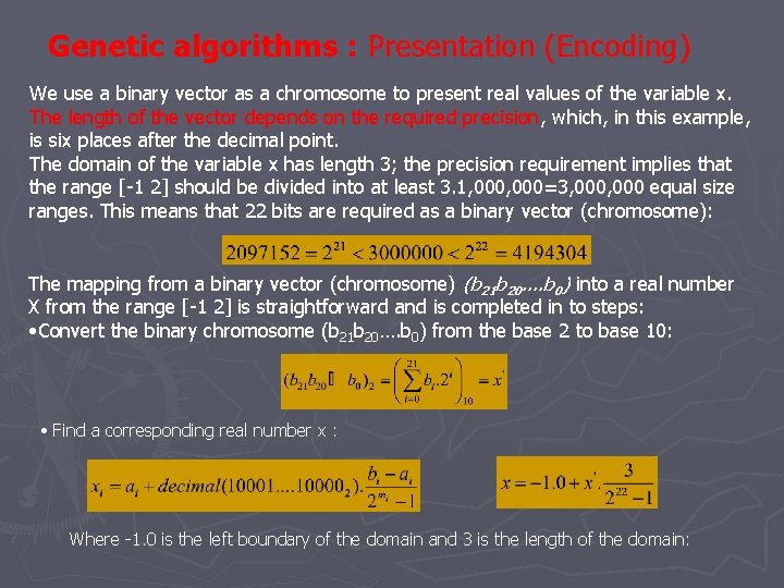
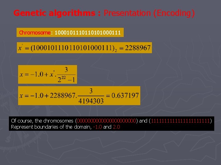
Genetic algorithms : Presentation (Encoding) We use a binary vector as a chromosome to present real values of the variable x. The length of the vector depends on the required precision, which, in this example, is six places after the decimal point. The domain of the variable x has length 3; the precision requirement implies that the range [-1 2] should be divided into at least 3. 1, 000=3, 000 equal size ranges. This means that 22 bits are required as a binary vector (chromosome): The mapping from a binary vector (chromosome) (b 21 b 20. . b 0) into a real number X from the range [-1 2] is straightforward and is completed in to steps: • Convert the binary chromosome (b 21 b 20…. b 0) from the base 2 to base 10: • Find a corresponding real number x : Where -1. 0 is the left boundary of the domain and 3 is the length of the domain:

Genetic algorithms : Presentation (Encoding) Chromosome: 100010110101000111 Of course, the chromosomes (00000000000) and (11111111111) Represent boundaries of the domain, -1. 0 and 2. 0

Genetic algorithms : Initial population The initialization process is very simple: we create a population of chromosomes, where each chromosome is is a binary vector of 22 bits. All 22 bits for each chromosome are initialized Randomly.

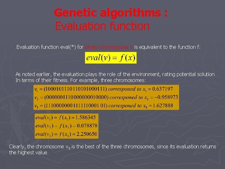
Genetic algorithms : Evaluation function eval(*) for binary chromosome v is equivalent to the function f: As noted earlier, the evaluation plays the role of the environment, rating potential solution In terms of their fitness. For example, three chromosomes: Clearly, the chromosome v 3 is the best of the three chromosomes, since its evaluation returns the highest value.

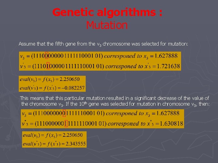
Genetic algorithms : Mutation Assume that the fifth gene from the v 3 chromosome was selected for mutation: This means that this particular mutation resulted in a significant decrease of the value of the chromosome v 3. If the 10 th gene was selected for mutation in chromosome v 3, then:

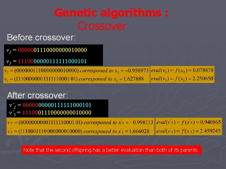
Genetic algorithms : Crossover Before crossover: v 2 = 000000111000010000 v 3 = 1110000000111111000101 After crossover: v’ 2 = 00000111111000101 v’ 3 = 1110000000010000 Note that the second offspring has a better evaluation than both of its parents.

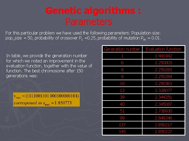
Genetic algorithms : Parameters For this particular problem we have used the following parameters: Population size: pop_size = 50, probability of crossover Pc =0. 25, probability of mutation Pm = 0. 01. In table, we provide the generation number for which we noted an improvement in the evaluation function, together with the value of function. The best chromosome after 150 generations was: Generation number Evaluation function 1 1. 441942 6 2. 250003 8 2. 250283 9 2. 250284 10 2. 250363 12 2. 328077 39 2. 344251 40 2. 345087 51 2. 738930 99 2. 849246 137 2. 850217 145 2. 850227

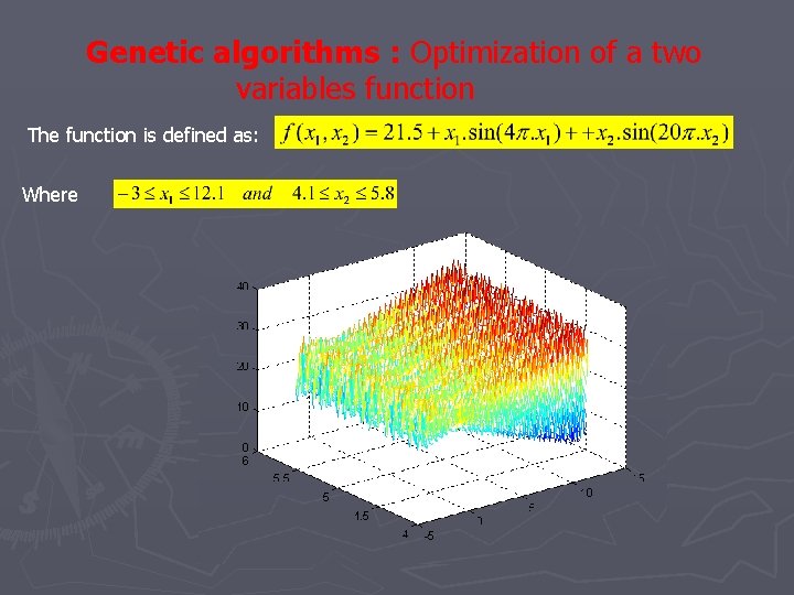
Genetic algorithms : Optimization of a two variables function The function is defined as: Where

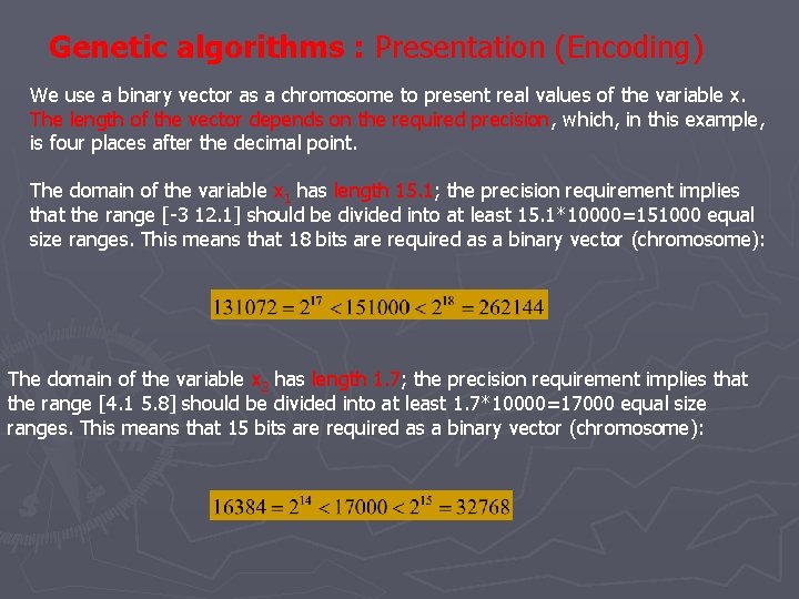
Genetic algorithms : Presentation (Encoding) We use a binary vector as a chromosome to present real values of the variable x. The length of the vector depends on the required precision, which, in this example, is four places after the decimal point. The domain of the variable x 1 has length 15. 1; the precision requirement implies that the range [-3 12. 1] should be divided into at least 15. 1*10000=151000 equal size ranges. This means that 18 bits are required as a binary vector (chromosome): The domain of the variable x 2 has length 1. 7; the precision requirement implies that the range [4. 1 5. 8] should be divided into at least 1. 7*10000=17000 equal size ranges. This means that 15 bits are required as a binary vector (chromosome):

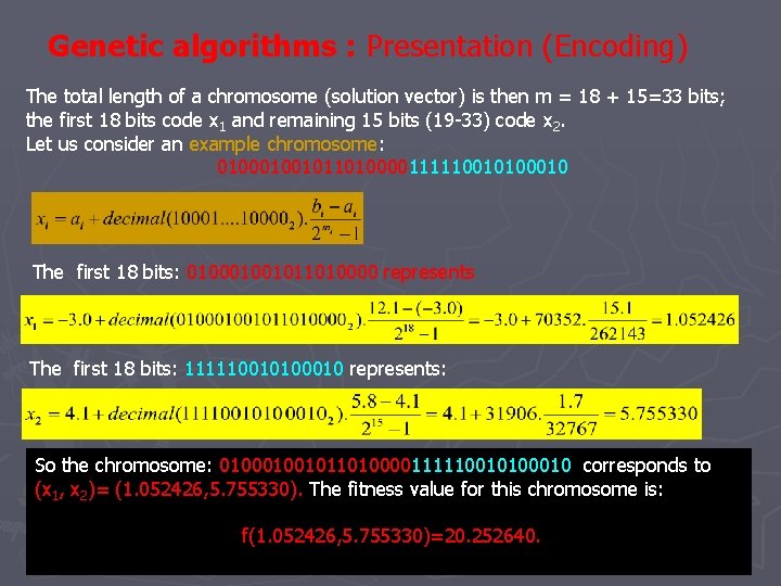
Genetic algorithms : Presentation (Encoding) The total length of a chromosome (solution vector) is then m = 18 + 15=33 bits; the first 18 bits code x 1 and remaining 15 bits (19 -33) code x 2. Let us consider an example chromosome: 01001011010000111110010100010 The first 18 bits: 01001011010000 represents The first 18 bits: 111110010100010 represents: So the chromosome: 01001011010000111110010100010 corresponds to (x 1, x 2)= (1. 052426, 5. 755330). The fitness value for this chromosome is: f(1. 052426, 5. 755330)=20. 252640.

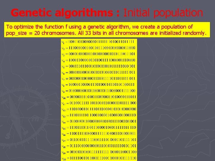
Genetic algorithms : Initial population To optimize the function f using a genetic algorithm, we create a population of pop_size = 20 chromosomes. All 33 bits in all chromosomes are initialized randomly.

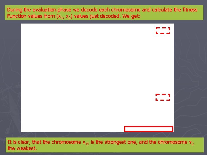
During the evaluation phase we decode each chromosome and calculate the fitness Function values from (x 1, x 2) values just decoded. We get: It is clear, that the chromosome v 15 is the strongest one, and the chromosome v 2 the weakest.

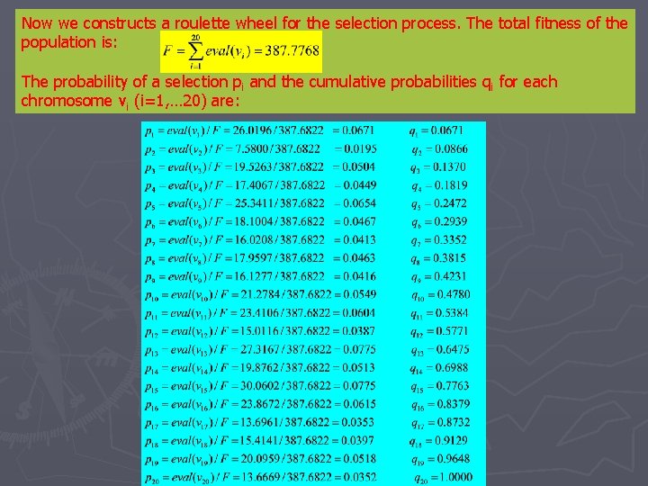
Now we constructs a roulette wheel for the selection process. The total fitness of the population is: The probability of a selection pi and the cumulative probabilities qi for each chromosome vi (i=1, … 20) are:

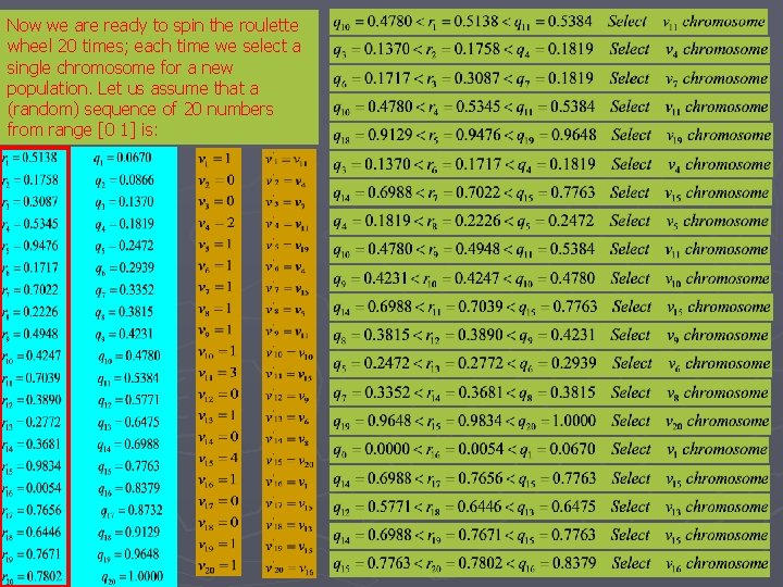
Now we are ready to spin the roulette wheel 20 times; each time we select a single chromosome for a new population. Let us assume that a (random) sequence of 20 numbers from range [0 1] is:

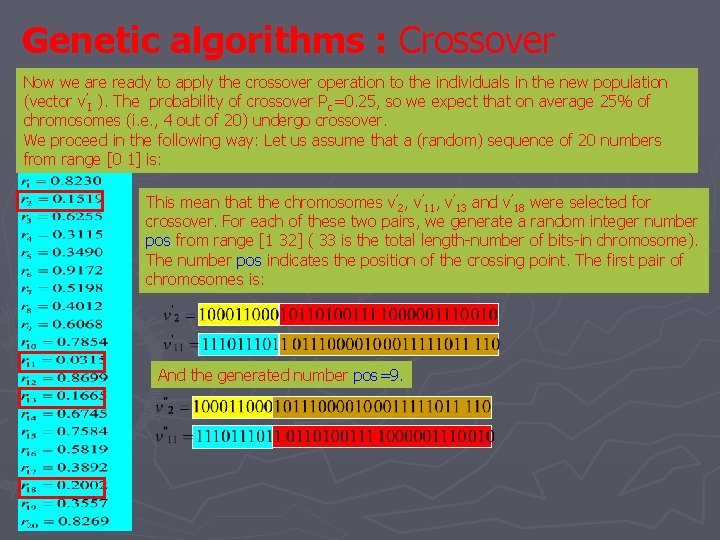
Genetic algorithms : Crossover Now we are ready to apply the crossover operation to the individuals in the new population (vector v’I ). The probability of crossover Pc=0. 25, so we expect that on average 25% of chromosomes (i. e. , 4 out of 20) undergo crossover. We proceed in the following way: Let us assume that a (random) sequence of 20 numbers from range [0 1] is: This mean that the chromosomes v’ 2, v’ 11, v’ 13 and v’ 18 were selected for crossover. For each of these two pairs, we generate a random integer number pos from range [1 32] ( 33 is the total length-number of bits-in chromosome). The number pos indicates the position of the crossing point. The first pair of chromosomes is: And the generated number pos=9.

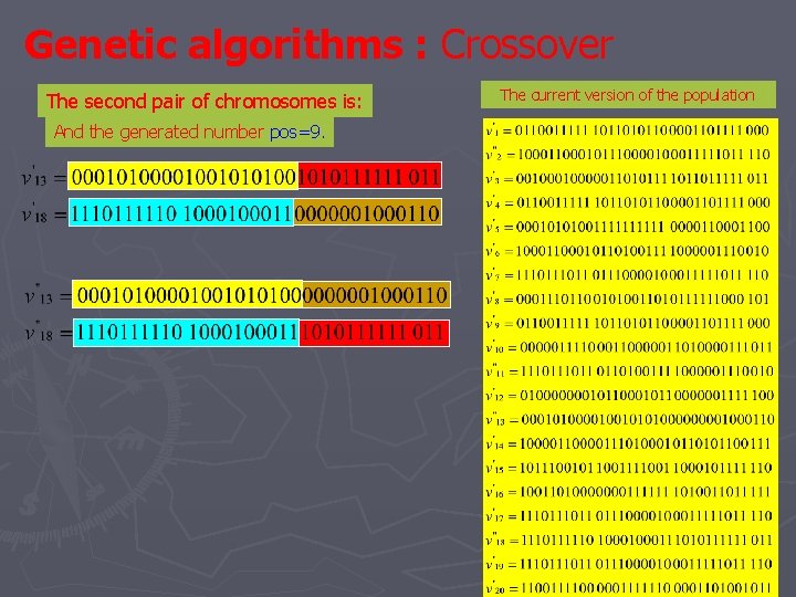
Genetic algorithms : Crossover The second pair of chromosomes is: And the generated number pos=9. The current version of the population

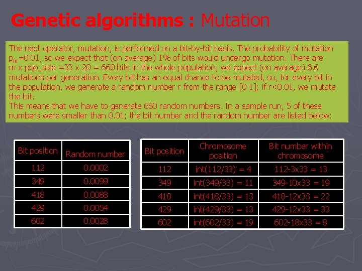
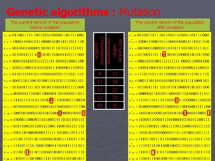
Genetic algorithms : Mutation The next operator, mutation, is performed on a bit-by-bit basis. The probability of mutation pm=0. 01, so we expect that (on average) 1% of bits would undergo mutation. There are m x pop_size =33 x 20 = 660 bits in the whole population; we expect (on average) 6. 6 mutations per generation. Every bit has an equal chance to be mutated, so, for every bit in the population, we generate a random number r from the range [0 1]; if r<0. 01, we mutate the bit. This means that we have to generate 660 random numbers. In a sample run, 5 of these numbers were smaller than 0. 01; the bit number and the random number are listed below: Random number Bit position Chromosome position Bit number within chromosome 112 0. 0002 112 int(112/33) = 4 112 -3 x 33 = 13 349 0. 0099 349 int(349/33) = 11 349 -10 x 33 = 19 418 0. 0088 418 int(418/33) = 13 418 -12 x 33 = 22 429 0. 0054 429 int(429/33) = 13 429 -12 x 33 = 33 602 0. 0028 602 int(602/33) = 19 602 -18 x 33 = 8 Bit position

Genetic algorithms : Mutation The current version of the population before mutation The current version of the population after mutation Bit number within chromosome Chromosome position 4 13 11 19 13 22 13 33 19 8

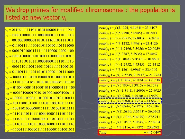
We drop primes for modified chromosomes : the population is listed as new vector vi:

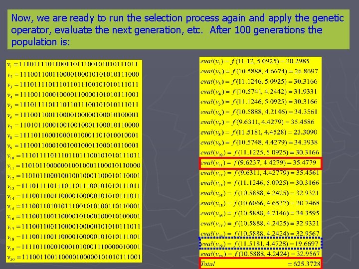
Now, we are ready to run the selection process again and apply the genetic operator, evaluate the next generation, etc. After 100 generations the population is:

Hybrid intelligent systems Evolutionary neural networks

Evolutionary neural networks n n Although neural networks are used for solving a variety of problems, they still have some limitations. One of the most common is associated with neural network training. The back-propagation learning algorithm cannot guarantee an optimal solution. In real-world applications, the back-propagation algorithm might converge to a set of sub-optimal weights from which it cannot escape. As a result, the neural network is often unable to find a desirable solution to a problem at hand.

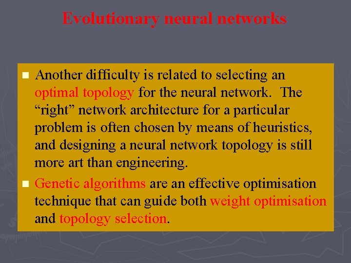
Evolutionary neural networks n n Another difficulty is related to selecting an optimal topology for the neural network. The “right” network architecture for a particular problem is often chosen by means of heuristics, and designing a neural network topology is still more art than engineering. Genetic algorithms are an effective optimisation technique that can guide both weight optimisation and topology selection.

Encoding a set of weights in a chromosome

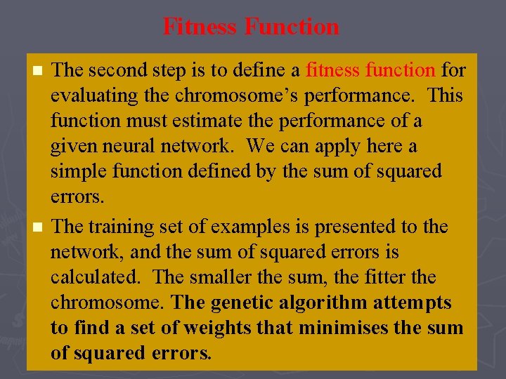
Fitness Function n n The second step is to define a fitness function for evaluating the chromosome’s performance. This function must estimate the performance of a given neural network. We can apply here a simple function defined by the sum of squared errors. The training set of examples is presented to the network, and the sum of squared errors is calculated. The smaller the sum, the fitter the chromosome. The genetic algorithm attempts to find a set of weights that minimises the sum of squared errors.

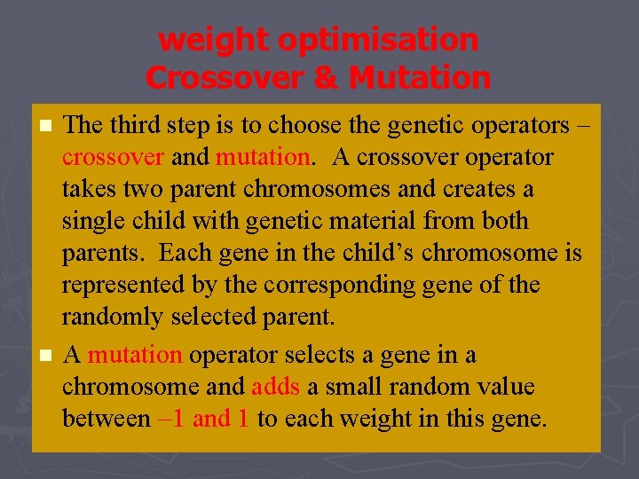
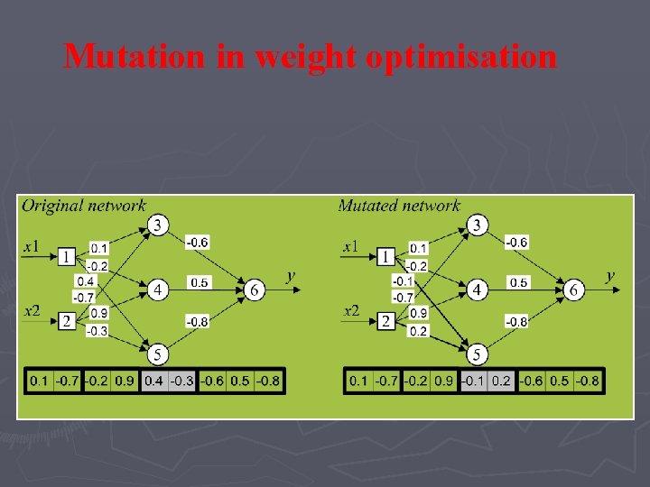
weight optimisation Crossover & Mutation n n The third step is to choose the genetic operators – crossover and mutation. A crossover operator takes two parent chromosomes and creates a single child with genetic material from both parents. Each gene in the child’s chromosome is represented by the corresponding gene of the randomly selected parent. A mutation operator selects a gene in a chromosome and adds a small random value between 1 and 1 to each weight in this gene.

Crossover in weight optimisation

Mutation in weight optimisation

Evolutionary neural networks: optimal topology Can genetic algorithms help us in selecting the network architecture? The architecture of the network (i. e. the number of neurons and their interconnections) often determines the success or failure of the application. Usually the network architecture is decided by trial and error; there is a great need for a method of automatically designing the architecture for a particular application. Genetic algorithms may well be suited for this task.

Evolutionary neural networks: optimal topology n n The basic idea behind evolving a suitable network architecture is to conduct a genetic search in a population of possible architectures. We must first choose a method of encoding a network’s architecture into a chromosome.

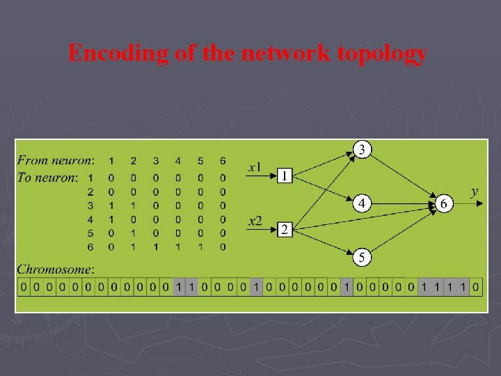
Encoding the network architecture n n n The connection topology of a neural network can be represented by a square connectivity matrix. Each entry in the matrix defines the type of connection from one neuron (column) to another (row), where 0 means no connection and 1 denotes connection for which the weight can be changed through learning. To transform the connectivity matrix into a chromosome, we need only to string the rows of the matrix together.

Encoding of the network topology

The cycle of evolving a neural network topology

Questions? Discussion? Suggestions ?