Digital Image Processing Using MATLAB Digital Image Processing

Digital Image Processing Using MATLAB®
 (a) 방법 I; (b) ~ (d) 방법")
Digital Image Processing Using MATLAB® (확대 그림) (a) 방법 I; (b) ~ (d) 방법 II (c) imshow(g, [ ])

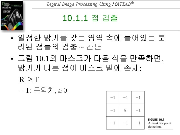
Digital Image Processing Using MATLAB® Chapter 10 Image Segmentation
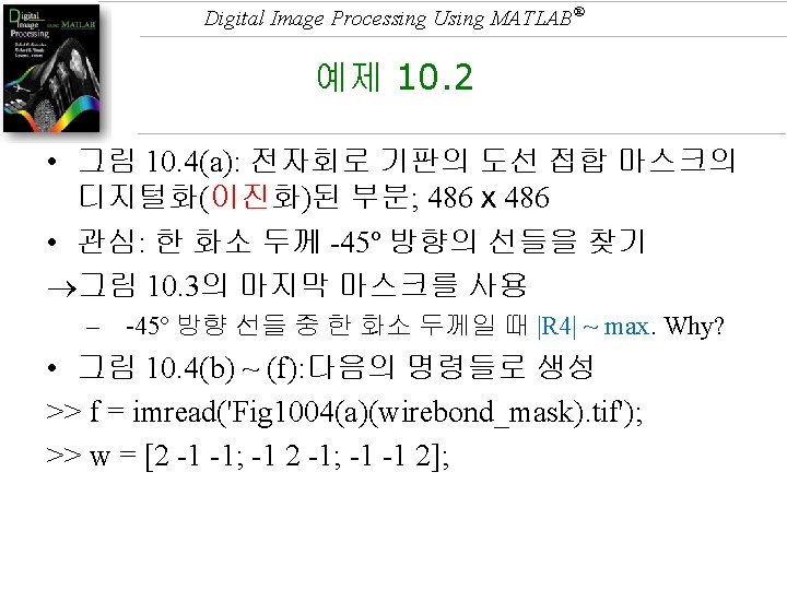
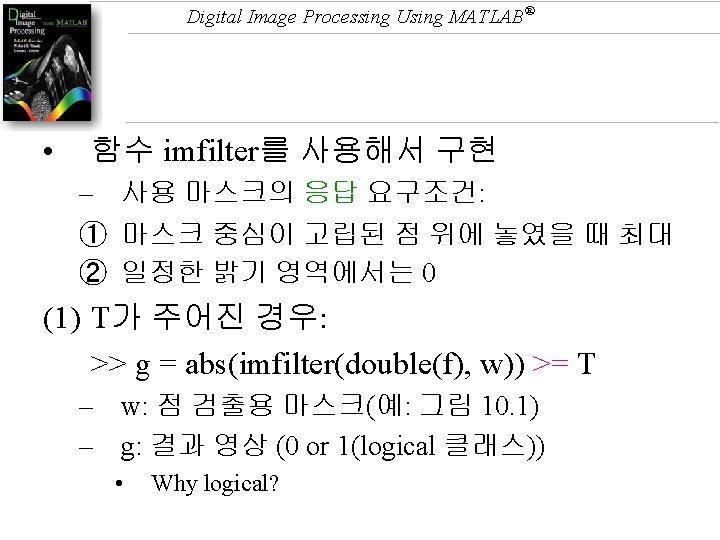
![Digital Image Processing Using MATLAB® >> g = imfilter(double(f), w); >> imshow(g, [ ])](http://slidetodoc.com/presentation_image_h2/6ae9ae44e97af0f6b426af5480bc71d1/image-22.jpg "Digital Image Processing Using MATLAB® >> g = imfilter(double(f), w); >> imshow(g, [ ])")
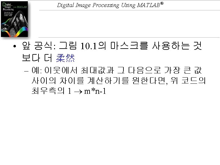
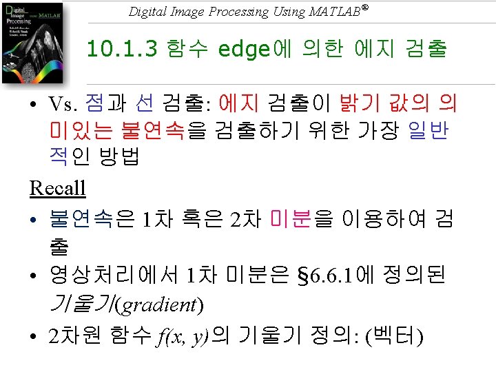
Digital Image Processing Using MATLAB® >> g = imfilter(double(f), w); >> imshow(g, [ ]) % 회색 톤 음값 >> gtop = g(1: 120, 1: 120); >> gtop = pixeldup(gtop, 4); >> figure, imshow(gtop, [ ]) >> gbot = g(end-119: end, end-119: end); >> gbot = pixeldup(gbot, 4); >> figure, imshow(gbot, [ ]) >> g = abs(g); >> figure, imshow(g, [ ]) >> T = max(g(: )); >> g = g >= T; >> figure, imshow(g) Fig. (b) Fig. (c) Fig. (d) Fig. (e) Fig. (f)

Digital Image Processing Using MATLAB®

Digital Image Processing Using MATLAB® 2차 미분과 노이즈 영향
 (출처: G & W,")
Digital Image Processing Using MATLAB® The Laplacian (2 nd-order derivative) (출처: G & W, 2002) • Isotropic for rotation increments of 90º and 45º, resp.

Digital Image Processing Using MATLAB® Chapter 10 Image Segmentation

Digital Image Processing Using MATLAB®
")
Digital Image Processing Using MATLAB® Sobel Edge 검출 • § 3. 5. 1 1) 그림 10. 5(b)의 좌, 우 마스크로 각각 영상 f를 필 터링(by imfilter) • BW = edge(I, 'sobel', thresh, direction) specifies the direction of detection for the Sobel method. direction is a string specifying whether to look for 'horizontal' or 'vertical' edges or 'both' (the default). 2) 각 필터링된 영상의 화소값을 제곱하여, 두 결과 를 더한 후, 제곱근 계산 (p. 418 공식) • 표 10. 1의 두 번째, 세 번째 에지 검출기도 같은 방법
 (출처: G &")
Digital Image Processing Using MATLAB® P 10. 8 (1 D Sobels) (출처: G & W, 2002) a b c d e f g h i 1 2 1 -1 0 g-a h-b i-c 1 e (g-a) + 2(h-b) + (i – c) = (g + 2 h + i) – (a + 2 b +c) • Show that the Sobel masks can be implemented by one pass of a diffrencing mask of the form [-1 0 1]' (or its vertical counterpart) followed by a smoothing mask of the form [1 2 1] (or its vertical counterpart).
")
Digital Image Processing Using MATLAB® 프류잇 Edge Detector • (Sobel의 설명과 비슷 skip)
")
Digital Image Processing Using MATLAB® 로버츠 Edge Detector • (Sobel의 설명과 비슷 skip)
 Detector • 가우스 함수:")
Digital Image Processing Using MATLAB® Lo. G (Laplacian of Gaussian) Detector • 가우스 함수: – – : 표준편차 – 영상을 흐릿하게 하는 정도 결정 • 이 함수의 라플라시안(r에 관한 2차 미분): Lo. G, Laplacian of a Gaussian

Digital Image Processing Using MATLAB® 출처: Gonzalez and Woods, 2002
")
Digital Image Processing Using MATLAB® Lo. G mask (출처: G & W, 2002)
![Digital Image Processing Using MATLAB® >> [g, t] = edge(f, 'log', [], 2); t](http://slidetodoc.com/presentation_image_h2/6ae9ae44e97af0f6b426af5480bc71d1/image-48.jpg "Digital Image Processing Using MATLAB® >> [g, t] = edge(f, 'log', [], 2); t")
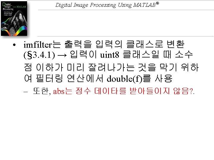
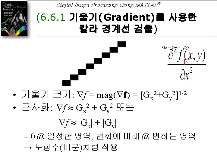
Digital Image Processing Using MATLAB® >> [g, t] = edge(f, 'log', [], 2); t = 0. 0071414 T=0때 histeq(f) 에 대해 숨겨진 경계선 개선. 반대는 약화.
); % Sobel - Lo. G 경우와 비교.")
Digital Image Processing Using MATLAB® • imshow(edge(f)); % Sobel - Lo. G 경우와 비교. 원인 분석!
![Digital Image Processing Using MATLAB® >> g = edge(f, 'log', [], 2); >> g](http://slidetodoc.com/presentation_image_h2/6ae9ae44e97af0f6b426af5480bc71d1/image-50.jpg "Digital Image Processing Using MATLAB® >> g = edge(f, 'log', [], 2); >> g")
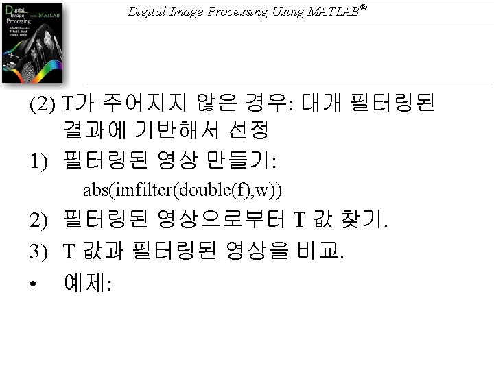
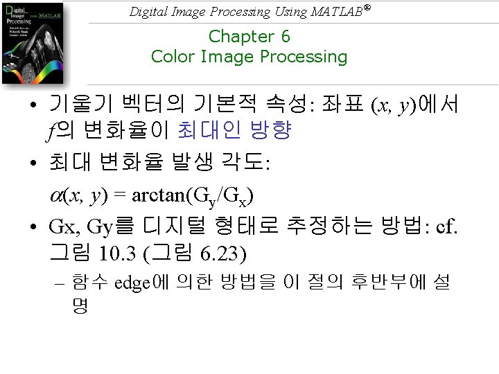
Digital Image Processing Using MATLAB® >> g = edge(f, 'log', [], 2); >> g = edge(f, 'canny', [], 2); % >> g = edge(f, ‘sobel', []);
![Digital Image Processing Using MATLAB® Zero-Crossing Detector • [g, t] = edge(f, 'zerocross', T,](http://slidetodoc.com/presentation_image_h2/6ae9ae44e97af0f6b426af5480bc71d1/image-51.jpg "Digital Image Processing Using MATLAB® Zero-Crossing Detector • [g, t] = edge(f, 'zerocross', T,")
Digital Image Processing Using MATLAB® Zero-Crossing Detector • [g, t] = edge(f, 'zerocross', T, H) – H: 규정된 필터 함수 • Gaussian + Laplacian + thr. + Z. C. det.

Digital Image Processing Using MATLAB® Edge finding by zero crossings (출처: Example 10. 15, G & W, 2002) • (b): Sobel image • (c) 27 x 27 smoothing mask ( = 5 pixels) • (e): Lo. G image Thinner i) (c) ? (Fig. 3. 34(b) ? ) ii) (d) ? • Zero-crossings: (f) & (g) i) Thr. : (e) (f) ii) Transition: (g)

Digital Image Processing Using MATLAB® What Gonzalez really used h= 1. 0 e-003 * Columns 1 through 12 0. 0096 0. 0114 0. 0137 0. 0114 0. 0139 0. 0173 0. 0137 0. 0173 0. 0219 0. 0166 0. 0214 0. 0274 0. 0201 0. 0262 0. 0338 0. 0241 0. 0316 0. 0406 0. 0283 0. 0373 0. 0475 0. 0327 0. 0429 0. 0540 0. 0369 0. 0480 0. 0596 0. 0406 0. 0525 0. 0642 0. 0438 0. 0560 0. 0675 0. 0461 0. 0586 0. 0697 0. 0475 0. 0602 0. 0710 0. 0480 0. 0607 0. 0714 0. 0475 0. 0602 0. 0710 0. 0461 0. 0586 0. 0697 0. 0438 0. 0560 0. 0675 0. 0406 0. 0525 0. 0642 0. 0369 0. 0480 0. 0596 0. 0327 0. 0429 0. 0540 0. 0283 0. 0373 0. 0475 0. 0241 0. 0316 0. 0406 0. 0201 0. 0262 0. 0338 0. 0166 0. 0214 0. 0274 0. 0137 0. 0173 0. 0219 0. 0114 0. 0139 0. 0173 0. 0096 0. 0114 0. 0137 0. 0166 0. 0214 0. 0274 0. 0345 0. 0424 0. 0505 0. 0581 0. 0647 0. 0697 0. 0732 0. 0750 0. 0758 0. 0760 0. 0761 0. 0760 0. 0758 0. 0750 0. 0732 0. 0697 0. 0647 0. 0581 0. 0505 0. 0424 0. 0345 0. 0274 0. 0214 0. 0166 0. 0201 0. 0262 0. 0338 0. 0424 0. 0515 0. 0602 0. 0675 0. 0728 0. 0756 0. 0759 0. 0745 0. 0722 0. 0703 0. 0695 0. 0703 0. 0722 0. 0745 0. 0759 0. 0756 0. 0728 0. 0675 0. 0602 0. 0515 0. 0424 0. 0338 0. 0262 0. 0201 0. 0241 0. 0316 0. 0406 0. 0505 0. 0602 0. 0684 0. 0741 0. 0761 0. 0741 0. 0687 0. 0613 0. 0539 0. 0484 0. 0464 0. 0484 0. 0539 0. 0613 0. 0687 0. 0741 0. 0761 0. 0741 0. 0684 0. 0602 0. 0505 0. 0406 0. 0316 0. 0241 0. 0283 0. 0373 0. 0475 0. 0581 0. 0675 0. 0741 0. 0760 0. 0722 0. 0626 0. 0484 0. 0321 0. 0169 0. 0062 0. 0023 0. 0062 0. 0169 0. 0321 0. 0484 0. 0626 0. 0722 0. 0760 0. 0741 0. 0675 0. 0581 0. 0475 0. 0373 0. 0283 0. 0327 0. 0429 0. 0540 0. 0647 0. 0728 0. 0761 0. 0722 0. 0600 0. 0397 0. 0135 -0. 0148 -0. 0402 -0. 0579 -0. 0642 -0. 0579 -0. 0402 -0. 0148 0. 0135 0. 0397 0. 0600 0. 0722 0. 0761 0. 0728 0. 0647 0. 0540 0. 0429 0. 0327 0. 0369 0. 0480 0. 0596 0. 0697 0. 0756 0. 0741 0. 0626 0. 0397 0. 0062 -0. 0348 -0. 0775 -0. 1152 -0. 1412 -0. 1504 -0. 1412 -0. 1152 -0. 0775 -0. 0348 0. 0062 0. 0397 0. 0626 0. 0741 0. 0756 0. 0697 0. 0596 0. 0480 0. 0369 0. 0406 0. 0525 0. 0642 0. 0732 0. 0759 0. 0687 0. 0484 0. 0135 -0. 0348 -0. 0918 -0. 1504 -0. 2015 -0. 2364 -0. 2488 -0. 2364 -0. 2015 -0. 1504 -0. 0918 -0. 0348 0. 0135 0. 0484 0. 0687 0. 0759 0. 0732 0. 0642 0. 0525 0. 0406 0. 0438 0. 0560 0. 0675 0. 0750 0. 0745 0. 0613 0. 0321 -0. 0148 -0. 0775 -0. 1504 -0. 2244 -0. 2884 -0. 3320 -0. 3475 -0. 3320 -0. 2884 -0. 2244 -0. 1504 -0. 0775 -0. 0148 0. 0321 0. 0613 0. 0745 0. 0750 0. 0675 0. 0560 0. 0438 0. 0461 0. 0586 0. 0697 0. 0758 0. 0722 0. 0539 0. 0169 -0. 0402 -0. 1152 -0. 2015 -0. 2884 -0. 3634 -0. 4143 -0. 4323 -0. 4143 -0. 3634 -0. 2884 -0. 2015 -0. 1152 -0. 0402 0. 0169 0. 0539 0. 0722 0. 0758 0. 0697 0. 0586 0. 0461 Columns 13 through 24 0. 0475 0. 0480 0. 0475 0. 0602 0. 0607 0. 0602 0. 0710 0. 0714 0. 0710 0. 0761 0. 0760 0. 0703 0. 0695 0. 0703 0. 0484 0. 0464 0. 0484 0. 0062 0. 0023 0. 0062 -0. 0579 -0. 0642 -0. 0579 -0. 1412 -0. 1504 -0. 1412 -0. 2364 -0. 2488 -0. 2364 -0. 3320 -0. 3475 -0. 3320 -0. 4143 -0. 4323 -0. 4143 -0. 4701 -0. 4898 -0. 5102 -0. 4898 -0. 4701 -0. 4143 -0. 4323 -0. 4143 -0. 3320 -0. 3475 -0. 3320 -0. 2364 -0. 2488 -0. 2364 -0. 1412 -0. 1504 -0. 1412 -0. 0579 -0. 0642 -0. 0579 0. 0062 0. 0023 0. 0062 0. 0484 0. 0464 0. 0484 0. 0703 0. 0695 0. 0703 0. 0760 0. 0761 0. 0760 0. 0714 0. 0710 0. 0602 0. 0607 0. 0602 0. 0475 0. 0480 0. 0475 Columns 25 through 27 0. 0137 0. 0114 0. 0096 0. 0173 0. 0139 0. 0114 0. 0219 0. 0173 0. 0137 0. 0274 0. 0214 0. 0166 0. 0338 0. 0262 0. 0201 0. 0406 0. 0316 0. 0241 0. 0475 0. 0373 0. 0283 0. 0540 0. 0429 0. 0327 0. 0596 0. 0480 0. 0369 0. 0642 0. 0525 0. 0406 0. 0675 0. 0560 0. 0438 0. 0697 0. 0586 0. 0461 0. 0710 0. 0602 0. 0475 0. 0714 0. 0607 0. 0480 0. 0710 0. 0602 0. 0475 0. 0697 0. 0586 0. 0461 0. 0675 0. 0560 0. 0438 0. 0642 0. 0525 0. 0406 0. 0596 0. 0480 0. 0369 0. 0540 0. 0429 0. 0327 0. 0475 0. 0373 0. 0283 0. 0406 0. 0316 0. 0241 0. 0338 0. 0262 0. 0201 0. 0274 0. 0214 0. 0166 0. 0219 0. 0173 0. 0137 0. 0173 0. 0139 0. 0114 0. 0137 0. 0114 0. 0096 0. 0461 0. 0586 0. 0697 0. 0758 0. 0722 0. 0539 0. 0169 -0. 0402 -0. 1152 -0. 2015 -0. 2884 -0. 3634 -0. 4143 -0. 4323 -0. 4143 -0. 3634 -0. 2884 -0. 2015 -0. 1152 -0. 0402 0. 0169 0. 0539 0. 0722 0. 0758 0. 0697 0. 0586 0. 0461 0. 0438 0. 0560 0. 0675 0. 0750 0. 0745 0. 0613 0. 0321 -0. 0148 -0. 0775 -0. 1504 -0. 2244 -0. 2884 -0. 3320 -0. 3475 -0. 3320 -0. 2884 -0. 2244 -0. 1504 -0. 0775 -0. 0148 0. 0321 0. 0613 0. 0745 0. 0750 0. 0675 0. 0560 0. 0438 0. 0406 0. 0525 0. 0642 0. 0732 0. 0759 0. 0687 0. 0484 0. 0135 -0. 0348 -0. 0918 -0. 1504 -0. 2015 -0. 2364 -0. 2488 -0. 2364 -0. 2015 -0. 1504 -0. 0918 -0. 0348 0. 0135 0. 0484 0. 0687 0. 0759 0. 0732 0. 0642 0. 0525 0. 0406 0. 0369 0. 0480 0. 0596 0. 0697 0. 0756 0. 0741 0. 0626 0. 0397 0. 0062 -0. 0348 -0. 0775 -0. 1152 -0. 1412 -0. 1504 -0. 1412 -0. 1152 -0. 0775 -0. 0348 0. 0062 0. 0397 0. 0626 0. 0741 0. 0756 0. 0697 0. 0596 0. 0480 0. 0369 0. 0327 0. 0429 0. 0540 0. 0647 0. 0728 0. 0761 0. 0722 0. 0600 0. 0397 0. 0135 -0. 0148 -0. 0402 -0. 0579 -0. 0642 -0. 0579 -0. 0402 -0. 0148 0. 0135 0. 0397 0. 0600 0. 0722 0. 0761 0. 0728 0. 0647 0. 0540 0. 0429 0. 0327 0. 0283 0. 0373 0. 0475 0. 0581 0. 0675 0. 0741 0. 0760 0. 0722 0. 0626 0. 0484 0. 0321 0. 0169 0. 0062 0. 0023 0. 0062 0. 0169 0. 0321 0. 0484 0. 0626 0. 0722 0. 0760 0. 0741 0. 0675 0. 0581 0. 0475 0. 0373 0. 0283 0. 0241 0. 0316 0. 0406 0. 0505 0. 0602 0. 0684 0. 0741 0. 0761 0. 0741 0. 0687 0. 0613 0. 0539 0. 0484 0. 0464 0. 0484 0. 0539 0. 0613 0. 0687 0. 0741 0. 0761 0. 0741 0. 0684 0. 0602 0. 0505 0. 0406 0. 0316 0. 0241 0. 0201 0. 0262 0. 0338 0. 0424 0. 0515 0. 0602 0. 0675 0. 0728 0. 0756 0. 0759 0. 0745 0. 0722 0. 0703 0. 0695 0. 0703 0. 0722 0. 0745 0. 0759 0. 0756 0. 0728 0. 0675 0. 0602 0. 0515 0. 0424 0. 0338 0. 0262 0. 0201 0. 0166 0. 0214 0. 0274 0. 0345 0. 0424 0. 0505 0. 0581 0. 0647 0. 0697 0. 0732 0. 0750 0. 0758 0. 0760 0. 0761 0. 0760 0. 0758 0. 0750 0. 0732 0. 0697 0. 0647 0. 0581 0. 0505 0. 0424 0. 0345 0. 0274 0. 0214 0. 0166

Digital Image Processing Using MATLAB® What the author used
 Threshold the Lo. G image (‘+’")
Digital Image Processing Using MATLAB® Approximating zero-crossings i) Threshold the Lo. G image (‘+’ = white; ‘-’ = black) Fig. (f) ii) Note the transitions btwn B & W in (f) Fig. (g) • The logic behind: Zero-crossings occur btwn + & - values of the Laplacian.
 vs. (g) • Zero-crossing edges")
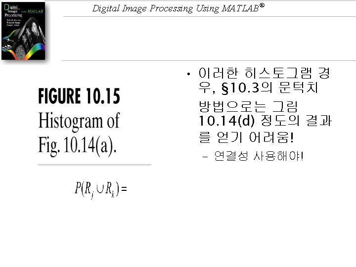
Digital Image Processing Using MATLAB® Figs. 10. 15 (b) vs. (g) • Zero-crossing edges are thinner than gradient edges. Attractive! • Noise reduction capabilities • However, – numerous closed loops (Spaghetti effect) – computation of zero crossings -- considerably more sophiscated techniques often are required to obtain acceptable results impractical

Digital Image Processing Using MATLAB® Result - 27 x 27 Lo. G mask // Lo. G() for(j= margin; j<m_n. Height-margin; j++){ for(i=margin ; i<m_n. Width-margin ; i++){ d. Temp = 0. ; // Note: margin = sizeofmask / 2 for(int x = - margin; x <= margin; x++) for(int y = -margin; y <= margin; y++) d. Temp += ptr. Sorce[j + x][i + y] * pn. Filter[n++]; p = (int)d. Temp + 127; // ? p >> ptr. Dest[j][i]; } }

Digital Image Processing Using MATLAB® Z. C. = Lo. G > Thr. > Transition Factors: 1. Offset value in Lo. G(): + 127? 2. Threshold value

Digital Image Processing Using MATLAB® What I used: width = 27; sigma = 5; h = fspecial('gaussian', width, sigma);

Digital Image Processing Using MATLAB®

Digital Image Processing Using MATLAB® Canny Edge Detector • The most powerful edge detector provided by function edge. finds edges by looking for local maxima of the gradient. (“Nonmaximum Suppression”) • uses two thresholds, to detect strong and weak edges, and includes the weak edges in the output only if they are connected to strong edges. (“Hysteresis Analysis”) therefore less likely than the others to be fooled by noise, and more likely to detect true weak edges. (에지로 검출된 것 중 노이즈는 제거하고, 약하더라도 진짜 에지는 검출해내 고)

Digital Image Processing Using MATLAB® 예제 10. 3 Sobel 검출기에 의한 경계선 추출 • 그림 10. 6(a) >> [gv, t] = edge(f, 'sobel', 'vertical'); >> imshow(gv) % 그림 (b) >> t t = 0. 0516 • 그림 (c): T = 0. 15 >> gv = edge(f, 'sobel', 0. 15, 'vertical'); • 그림 (d): 수평 + 수직 에지 >> gv = edge(f, 'sobel', 0. 15);
: Results of computing edges at 45º")
Digital Image Processing Using MATLAB® • 그림 (e): Results of computing edges at 45º >> w 45 = [-1 -1 2; -1 2 -1; 2 -1 -1]; >> imshow(imfilter(f, w 45)); • 그림 (f): -45º

Digital Image Processing Using MATLAB®

Digital Image Processing Using MATLAB® -2 -1 -1 0 0 1 2 • Vs. w 45 >> f_w 45 = imfilter(f, w 45); >> w 45 b = [-2 -1 0; -1 0 1; 0 1 2] >> imshow(f_w 45, []) >> f_w 45 b = imfilter(f, w 45 b);
) >> w_45 b")
Digital Image Processing Using MATLAB® >> imshow(im 2 bw(f_w 45 b)) >> w_45 b = [0 -1 -2; 1 0 -1; 2 1 0] w_45 b = 0 -1 -2 1 0 -1 2 1 0 >> f_w_45 b = imfilter(f, w_45 b); >> imshow(im 2 bw(f_w_45 b))
![Digital Image Processing Using MATLAB® (자동 모드) • 그림 10. 7(a): >> [g_sobel, ts]](http://slidetodoc.com/presentation_image_h2/6ae9ae44e97af0f6b426af5480bc71d1/image-69.jpg "Digital Image Processing Using MATLAB® (자동 모드) • 그림 10. 7(a): >> [g_sobel, ts]")
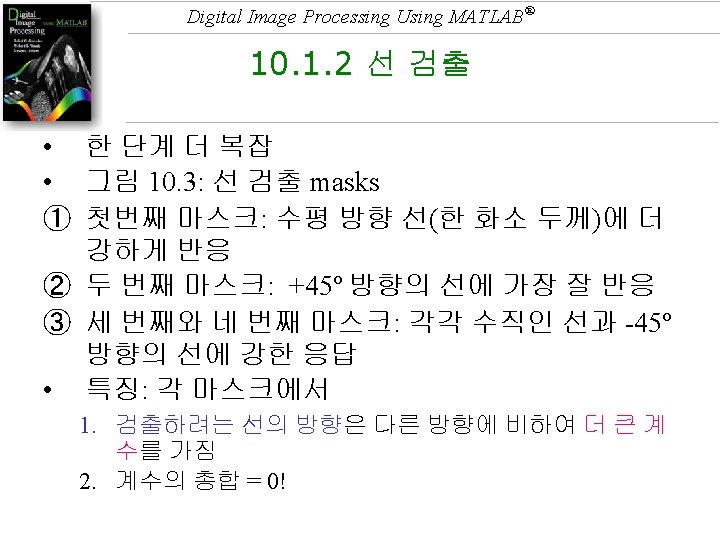
Digital Image Processing Using MATLAB® (자동 모드) • 그림 10. 7(a): >> [g_sobel, ts] = edge(f, 'sobel'); % ts = 0. 074 • 그림 10. 7(c): default sigma = 2. 0 >> [g_log, tlog] = edge(f, 'log'); % tlog = 0. 0025 • 그림 10. 7(e): default sigma = 1. 0 >> [g_canny, tc] = edge(f, 'canny'); % tc = [0. 019, 0. 047] (T 1 = 0. 4 * T 2)
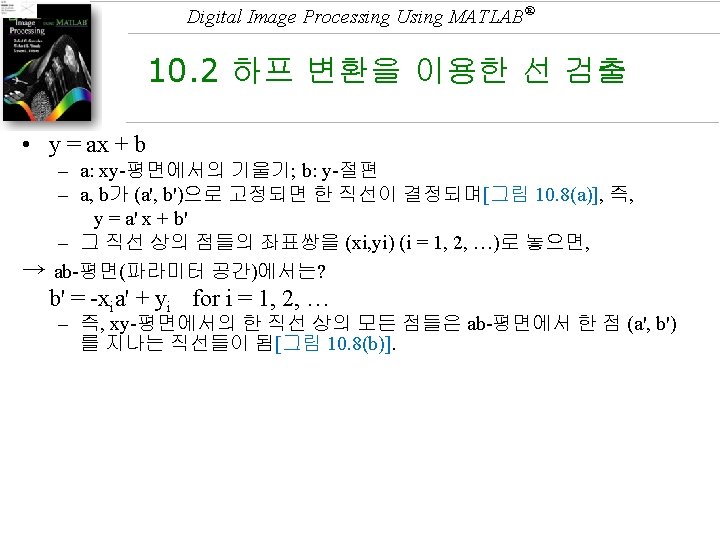

Digital Image Processing Using MATLAB® xy-평면 직선 상 점 ab-평면 교차 직선

Digital Image Processing Using MATLAB® 문제: 직선식 유도 • y = ax + b x cos + y sin = • Ans) – Hint: a, b ~ f( , )로 표현해서 제거
 + 1); • y = linspace(a,")
Digital Image Processing Using MATLAB® linspace(-90, 0, ceil(90/dtheta) + 1); • y = linspace(a, b, n) generates a row vector y of n points linearly spaced between and including a and b.

Digital Image Processing Using MATLAB® fliplr • Flip matrices left-right • Example: If A is the 3 -by-2 matrix, A = 1 4 2 5 3 6 then fliplr(A) produces 4 1 5 2 6 3
 (GW 2002)")
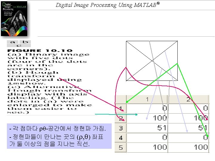
Digital Image Processing Using MATLAB® Example 10. 7 (Eq. 10. 2 -3) (GW 2002) (cf. 교재 그림 10. 10) • To pass through pt 2 in (a): [°] 0 45 90 0 1/ 2 1 – cf. Fig. (b) • To pass through pts 1, 3, 5: – pt A in (c) = 0, = -45° (pt B는 2, 3, 4) • (d) Reflective adjacency ( , change sign at ± 90°)
![Digital Image Processing Using MATLAB® 예제 10. 5 >>imshow(theta, rho, H, [], 'notruesize'), axis](http://slidetodoc.com/presentation_image_h2/6ae9ae44e97af0f6b426af5480bc71d1/image-80.jpg "Digital Image Processing Using MATLAB® 예제 10. 5 >>imshow(theta, rho, H, [], 'notruesize'), axis")
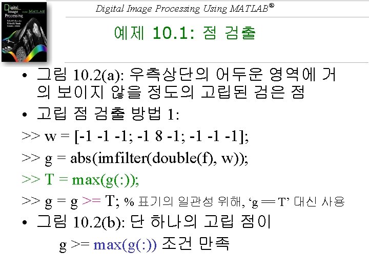
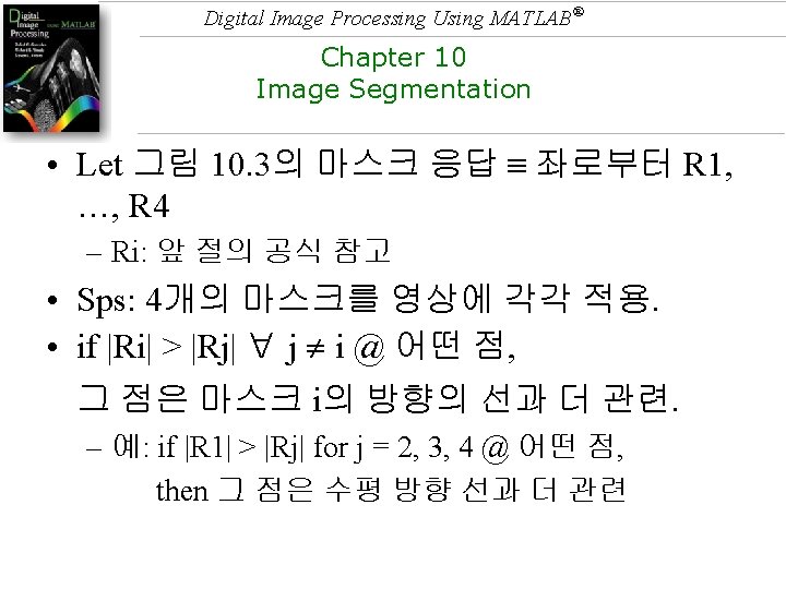
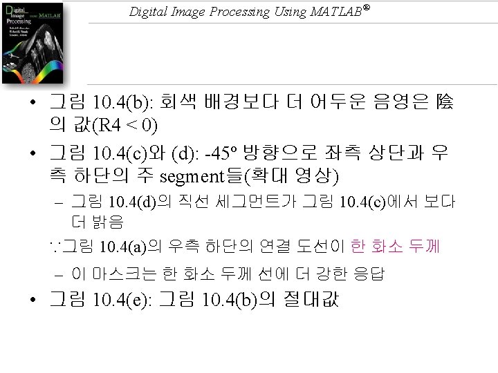
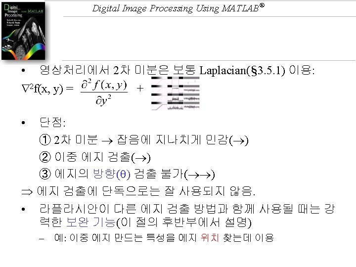
Digital Image Processing Using MATLAB® 예제 10. 5 >>imshow(theta, rho, H, [], 'notruesize'), axis on, axis normal • 그림 10. 10(a): 간단한 이진 영상 • 그림 10. 10(b): Hough 변환 결과 >> H = hough(f); >> imshow(H, [ ]) • 그림 10. 10(c): 축에 레이블 표시 + 더 큰 그림: >> [H, theta, rho] = hough(f); >> imshow(theta, rho, H, [], ‘n’); >> axis on, axis normal >> xlabel('theta'), ylabel('rho')

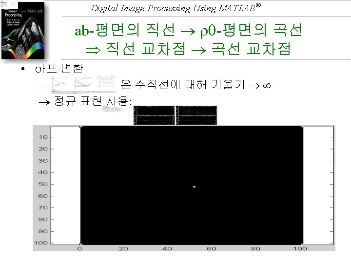
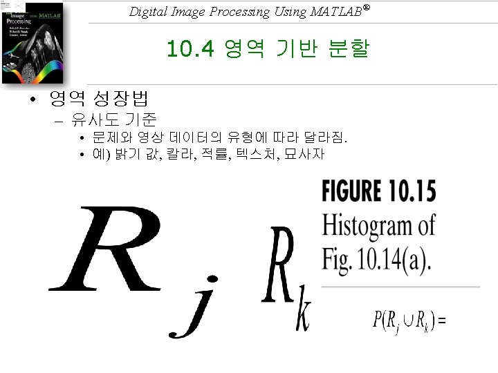
Digital Image Processing Using MATLAB® 10. 2 하프 변환을 이용한 선 검출 • 하프 변환의 예

Digital Image Processing Using MATLAB® xy-평면 구현하기 -- in hough. m … theta = linspace(-90, 0, ceil(90/dtheta) + 1); theta = [theta –fliplr(theta(2: end – 1))]; D = sqrt((M - 1)^2 + (N - 1)^2); q = ceil(D/drho); nrho = 2*q - 1; rho = linspace(-q*drho, nrho); [x, y, val] = find(f); x = x - 1; y = y - 1; [-90 -89 … 1 0] [-90 … 0 1 … 89] D = 141. 4 q = 142 [-142 … 0 … 142] x=[1 101 52 1 101]' y = [1 1 52 101]' val = [1 1 1]'

Digital Image Processing Using MATLAB® hough. m: draws five sinusoidal functions inside the dotted box below. image (0, 100) -142 max = 142 (100, 0) = [-90, 90] (100, 100) -90 142 0 90
/1000) first = (k -")
Digital Image Processing Using MATLAB® for k = 1: ceil(length(val)/1000) first = (k - 1)*1000 + 1; last = min(first+999, length(x)); x_matrix = repmat(x(first: last), 1, ntheta); y_matrix = repmat(y(first: last), 1, ntheta); val_matrix = repmat(val(first: last), 1, ntheta); theta_matrix = repmat(theta, size(x_matrix, 1)*pi/180; first = 1 last = 5

Digital Image Processing Using MATLAB® rho: 283 values theta: 180 values
![Digital Image Processing Using MATLAB® function [r, c, hnew] = houghpeaks(h, numpeaks, threshold, nhood)](http://slidetodoc.com/presentation_image_h2/6ae9ae44e97af0f6b426af5480bc71d1/image-88.jpg "Digital Image Processing Using MATLAB® function [r, c, hnew] = houghpeaks(h, numpeaks, threshold, nhood)")
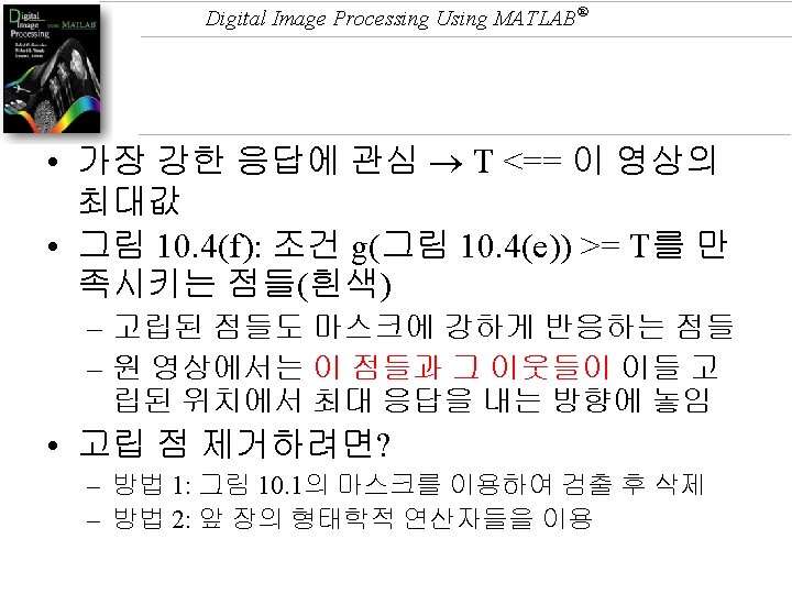
Digital Image Processing Using MATLAB® function [r, c, hnew] = houghpeaks(h, numpeaks, threshold, nhood) %HOUGHPEAKS Detect peaks in Hough transform. % [R, C, HNEW] = HOUGHPEAKS(H, NUMPEAKS, THRESHOLD, NHOOD) detects % peaks in the Hough transform matrix H. NUMPEAKS specifies the % maximum number of peak locations to look for. Values of H below % THRESHOLD will not be considered to be peaks. NHOOD is a % two-element vector specifying the size of the suppression % neighborhood. This is the neighborhood around each peak that is % set to zero after the peak is identified. The elements of NHOOD % must be positive, odd integers. R and C are the row and column % coordinates of the identified peaks. HNEW is the Hough transform % with peak neighborhood suppressed. %

Digital Image Processing Using MATLAB® % If NHOOD is omitted, it defaults to the smallest odd values >= % size(H)/50. If THRESHOLD is omitted, it defaults to % 0. 5*max(H(: )). If NUMPEAKS is omitted, it defaults to 1.

Digital Image Processing Using MATLAB® sub 2 ind • Single index from subscripts • IND = sub 2 ind(siz, I, J) returns the linear index equivalent to the row and column subscripts I and J for a matrix of size siz. • siz is a 2 -element vector, where siz(1) is the number of rows and siz(2) is the number of columns.

Digital Image Processing Using MATLAB® Examples: Create a 3 -by-4 -by-2 array, A. A = [17 24 1 8; 2 22 7 14; 4 6 13 20]; A(: , 2) = A - 10 A(: , 1) = 17 24 1 8 2 22 7 14 4 6 13 20 A(: , 2) = 7 14 -9 -2 -8 12 -3 4 -6 -4 3 10 The value at row 2, column 1, page 2 of the array is -8. >> A(2, 1, 2) ans = -8 To convert A(2, 1, 2) into its equivalent single subscript, use sub 2 ind. >> sub 2 ind(size(A), 2, 1, 2) ans = 14 >> A(14) ans = -8
![Digital Image Processing Using MATLAB® >> [r, c] = houghpeaks(H, 6); >> hold on](http://slidetodoc.com/presentation_image_h2/6ae9ae44e97af0f6b426af5480bc71d1/image-92.jpg "Digital Image Processing Using MATLAB® >> [r, c] = houghpeaks(H, 6); >> hold on")
Digital Image Processing Using MATLAB® >> [r, c] = houghpeaks(H, 6); >> hold on >> plot(theta(c), rho(r), 'linestyle', 'none', 'marker', 's', 'color', 'w')

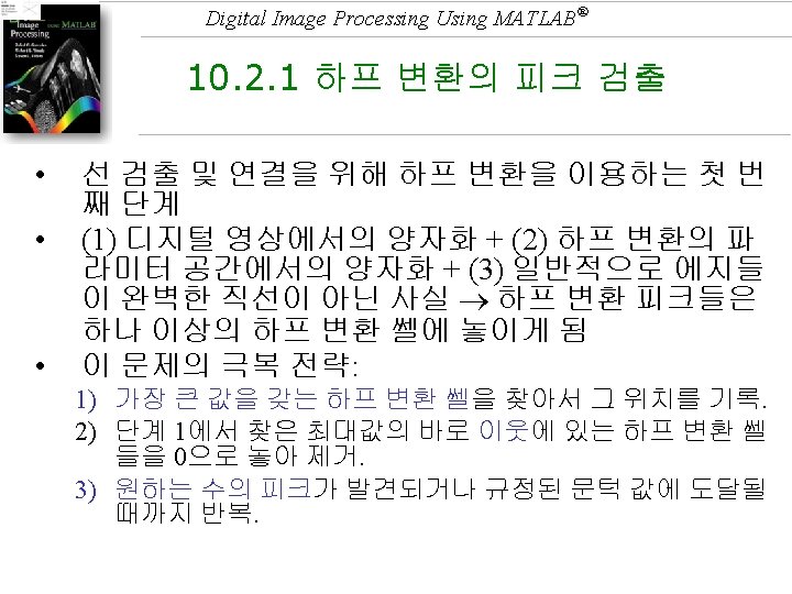
Digital Image Processing Using MATLAB® 10. 2. 2 하프 변환의 선 검출 및 연결 • houghpixels. m: peak에 기여한 화소들의 위 치 찾기 • houghlines. m: houghpixels로 찾은 화소들을 선분으로 그룹화
의 이진 영상에서")
Digital Image Processing Using MATLAB® 예제 10. 6 • 그림 10. 7(f)의 이진 영상에서 선분들을 찾 기 위해 함수 hough, houghpeaks, houghlines 를 사용 • >> xlabel('theta'), ylabel('rho') >> [r, c] = houghpeaks(H, 5); >> hold on >> plot(theta(c), rho(r), 'linestyle', 'none', 'marker', 's', 'color', 'w')
")
Digital Image Processing Using MATLAB® 그림 10. 11(a)
 >>")
Digital Image Processing Using MATLAB® >> lines = houghlines(g_canny_best, theta, rho, r, c) >> figure, imshow(g_canny_best), hold on
 xy = [lines(k).")
Digital Image Processing Using MATLAB® >> for k = 1: length(lines) xy = [lines(k). point 1; lines(k). point 2]; plot(xy(: , 2), xy(: , 1), 'Linewidth', 4, 'Color', [. 6. 6. 6]); end

Digital Image Processing Using MATLAB®

Digital Image Processing Using MATLAB® 10. 2. 2 하프 변환의 선 검출 및 연결

Digital Image Processing Using MATLAB® HW: 의미있는 선분 찾기
; >> f(30, 30: 60)")
Digital Image Processing Using MATLAB® >> f = zeros(100, 100); >> f(30, 30: 60) = 1; >> f(60, 30: 60) = 1; >> f(30: 60, 30) = 1; >> f(30: 60, 60) = 1; g = f; [M N] = size(g); [H, theta, rho] = hough(g, 1, . 5); % dtheta = 1, drho = 1 figure(1), subplot(3, 1, 1); imshow(theta, rho, H, [], 'n'); axis on, axis normal xlabel('theta'), ylabel('rho') [r, c] = houghpeaks(H, 4); hold on plot(theta(c), rho(r), 'linestyle', 'none', 'marker', 's', 'color', 'w') lines = my. Houghlines(g, theta, rho, r, c, 20, 10, N) % defaults: fillgap = 20, minlength = 40 subplot(3, 1, 2); imshow(g) subplot(3, 1, 3); imshow(g) hold on for k = 1: length(lines) xy = [lines(k). point 1; lines(k). point 2]; plot(xy(: , 2), xy(: , 1), 'linewidth', 3, 'color', [0. 3 0 0. 3]); end

Digital Image Processing Using MATLAB®

Digital Image Processing Using MATLAB® 5º, 40º
![Digital Image Processing Using MATLAB® [r, c] = houghpeaks(H, 20);](http://slidetodoc.com/presentation_image_h2/6ae9ae44e97af0f6b426af5480bc71d1/image-104.jpg "Digital Image Processing Using MATLAB® [r, c] = houghpeaks(H, 20);")
Digital Image Processing Using MATLAB® [r, c] = houghpeaks(H, 20);


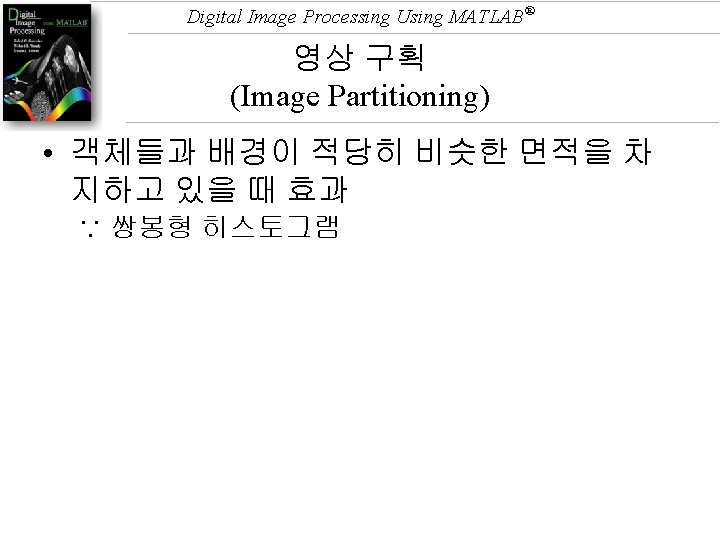
Digital Image Processing Using MATLAB® • Bimodal 쉬움.
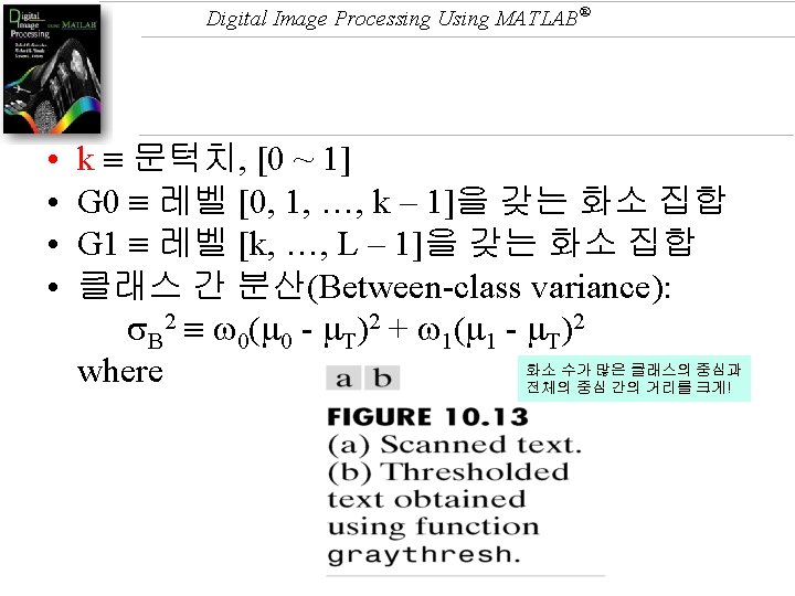
; B 2 = 0( 0")
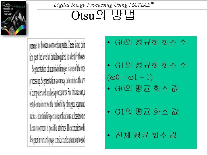
Digital Image Processing Using MATLAB® • T = graythresh(f); B 2 = 0( 0 - T)2 + 1( 1 - T)2 를 최대화 시키는 k를 계산 – T ~ [0, 1] 반환

Digital Image Processing Using MATLAB® 예제 10. 7 전역적 문턱치 처리 -- 반복적 방법 & Otsu 방법 T 1 = 0. 5 * (double(min(f(: )) + max(f(: )))); done = false; while ~done g = f >= T 1; Tnext = 0. 5 * (mean(f(g)) + mean(f(~g))); done = abs(T 1 - Tnext) < 0. 5; T 1 = Tnext; end figure(1), subplot(1, 2, 1); imshow(g); T 2 = graythresh(f); if class(f) == 'uint 8' T 2 = T 2 * 255; end g = f >= T 2; subplot(1, 2, 2), imshow(g) T 1 = 101. 47 T 2 = 101 거의 같은 결과

Digital Image Processing Using MATLAB®

Digital Image Processing Using MATLAB® Example 10. 11 Segmentation using an estimated global threshold (GW 2002) T(Final = 3) = 125. 4
 Original image, (b) Gray image,")
Digital Image Processing Using MATLAB® 차이가 분명한 경우: (a) Original image, (b) Gray image, (c) 방법 I, (d) 방법 II
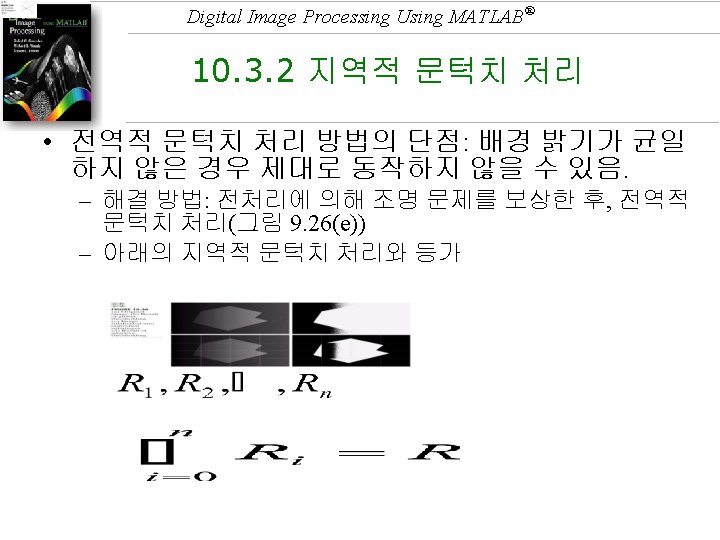

Digital Image Processing Using MATLAB® 적응적 문턱치 처리
) (GW 2002)")
Digital Image Processing Using MATLAB® Example 10. 12 (Fig. 10. 27 (d)) (GW 2002) • could not be thresholded effectively with a single T (b) manually placed T in the valley (Fig. 10. 27(e)) (c) subdivision(영상 구획)

Digital Image Processing Using MATLAB®

Digital Image Processing Using MATLAB® • 목표: 둘레 링 제거
 •")
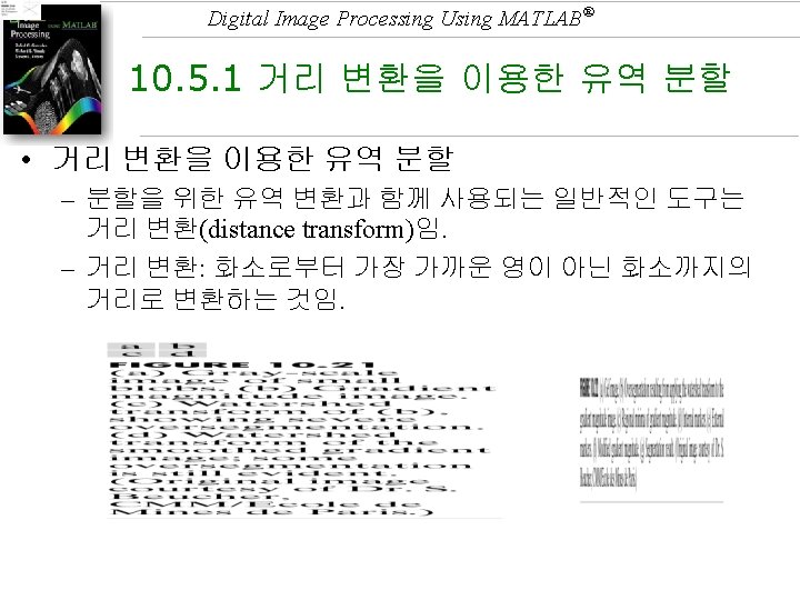
Digital Image Processing Using MATLAB® • 거리변환 D = bwdist(f) •

Digital Image Processing Using MATLAB® 예제 10. 10 • 거리 변환을 이용한 유역 분할

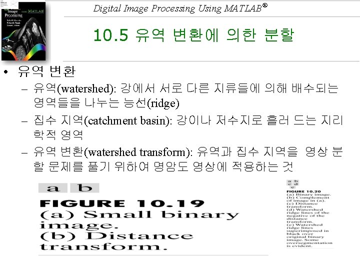
Digital Image Processing Using MATLAB® 10. 5 유역 변환에 의한 분할 • 마커-제어 유역 분할
- Slides: 146