Digital Image Processing Lecture 7 Geometric Transformation March

Digital Image Processing Lecture 7: Geometric Transformation March 16, 2005 Prof. Charlene Tsai Digital Image Processing Lecture 7

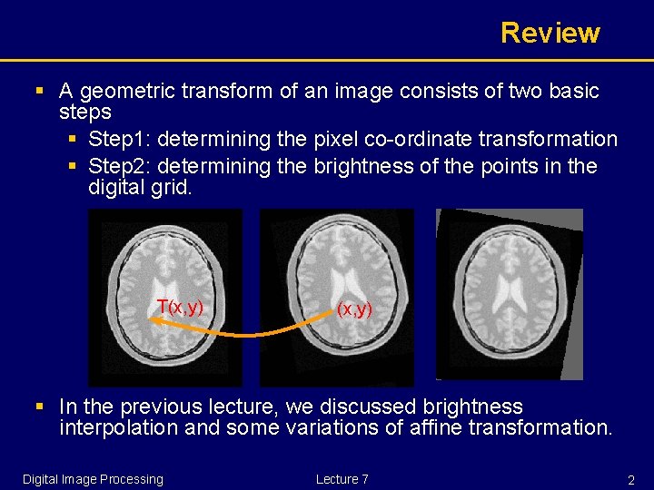
Review § A geometric transform of an image consists of two basic steps § Step 1: determining the pixel co-ordinate transformation § Step 2: determining the brightness of the points in the digital grid. T(x, y) § In the previous lecture, we discussed brightness interpolation and some variations of affine transformation. Digital Image Processing Lecture 7 2

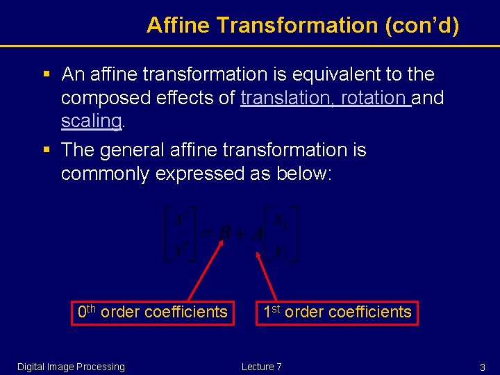
Affine Transformation (con’d) § An affine transformation is equivalent to the composed effects of translation, rotation and scaling. § The general affine transformation is commonly expressed as below: 0 th order coefficients Digital Image Processing 1 st order coefficients Lecture 7 3

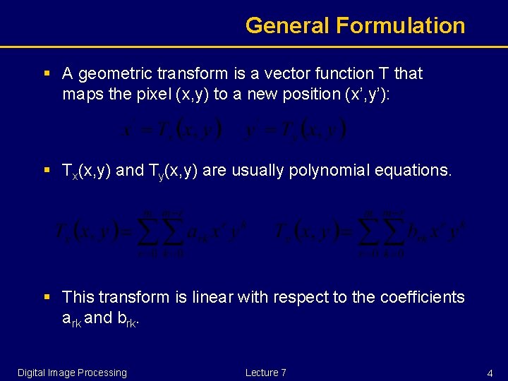
General Formulation § A geometric transform is a vector function T that maps the pixel (x, y) to a new position (x’, y’): § Tx(x, y) and Ty(x, y) are usually polynomial equations. § This transform is linear with respect to the coefficients ark and brk. Digital Image Processing Lecture 7 4

Finding Coefficients § How to find ark and brk, which are often unknown? § Finding pairs of corresponding points (x, y), (x’, y’) in both images, § Determining ark and brk by solving a set of linear equations. § More points than coefficients are usually used to get robustness. Least-squares fitting is often used. Digital Image Processing Lecture 7 5

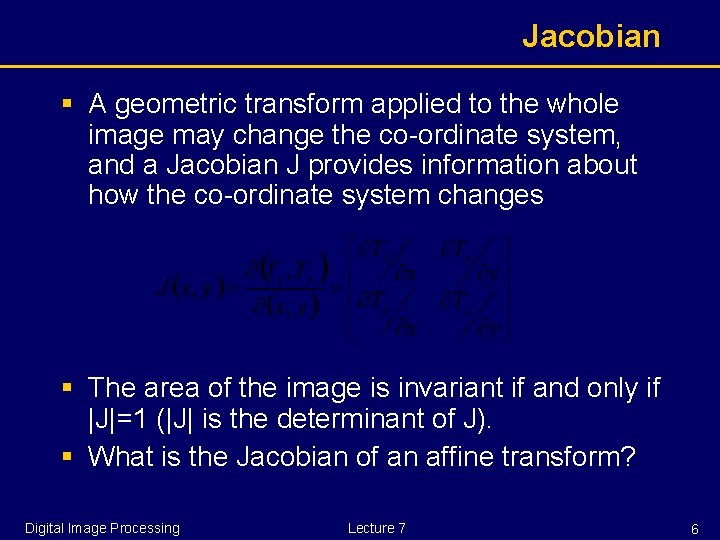
Jacobian § A geometric transform applied to the whole image may change the co-ordinate system, and a Jacobian J provides information about how the co-ordinate system changes § The area of the image is invariant if and only if |J|=1 (|J| is the determinant of J). § What is the Jacobian of an affine transform? Digital Image Processing Lecture 7 6

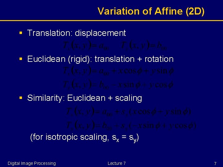
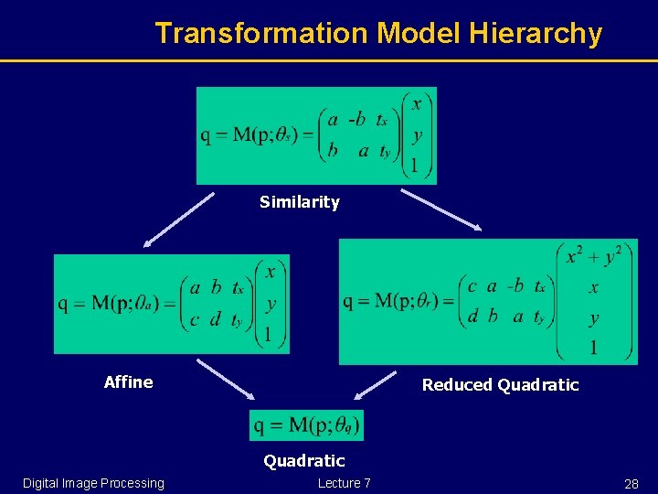
Variation of Affine (2 D) § Translation: displacement § Euclidean (rigid): translation + rotation § Similarity: Euclidean + scaling (for isotropic scaling, sx = sy) Digital Image Processing Lecture 7 7

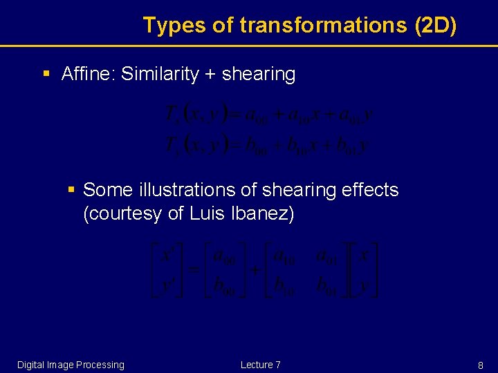
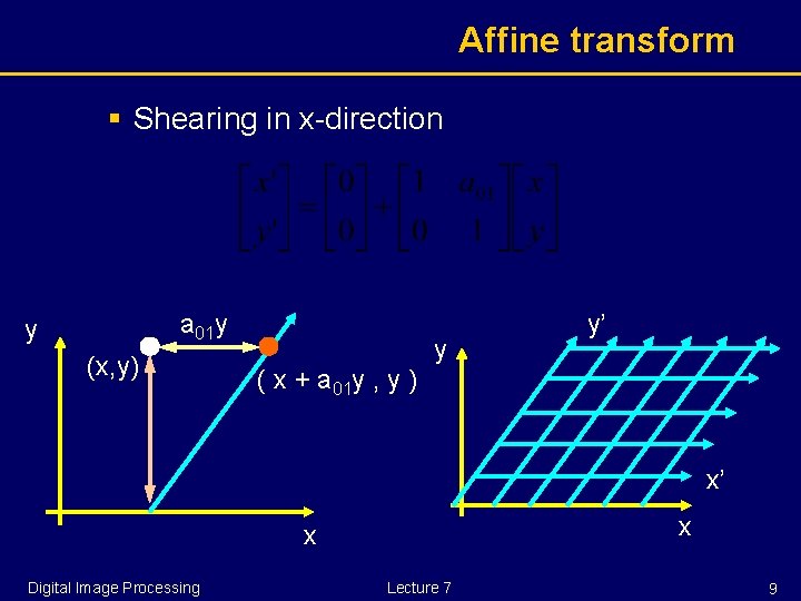
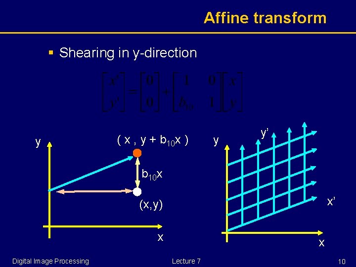
Types of transformations (2 D) § Affine: Similarity + shearing § Some illustrations of shearing effects (courtesy of Luis Ibanez) Digital Image Processing Lecture 7 8

Affine transform § Shearing in x-direction a 01 y y (x, y) y y’ ( x + a 01 y , y ) x’ x x Digital Image Processing Lecture 7 9

Affine transform § Shearing in y-direction y ( x , y + b 10 x ) y y’ b 10 x x’ (x, y) x Digital Image Processing x Lecture 7 10

Invariant Properties § Translation: § Euclidean: § Similarity: § Affine: Digital Image Processing Lecture 7 11

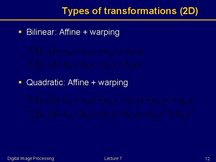
Types of transformations (2 D) § Bilinear: Affine + warping § Quadratic: Affine + warping Digital Image Processing Lecture 7 12

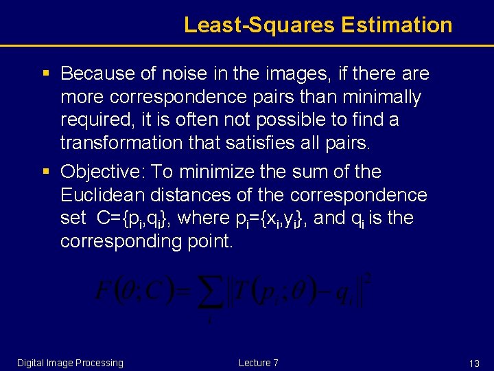
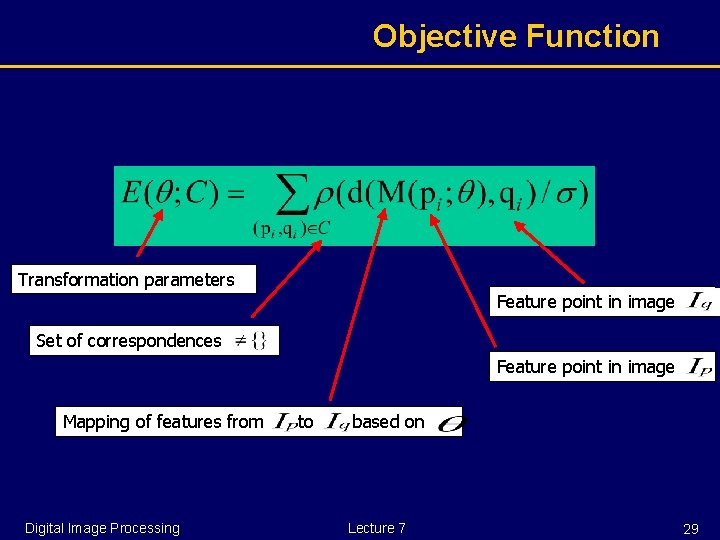
Least-Squares Estimation § Because of noise in the images, if there are more correspondence pairs than minimally required, it is often not possible to find a transformation that satisfies all pairs. § Objective: To minimize the sum of the Euclidean distances of the correspondence set C={pi, qi}, where pi={xi, yi}, and qi is the corresponding point. Digital Image Processing Lecture 7 13

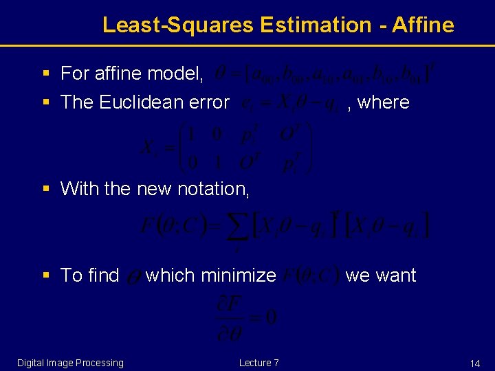
Least-Squares Estimation - Affine § For affine model, § The Euclidean error , where § With the new notation, § To find Digital Image Processing which minimize Lecture 7 we want 14

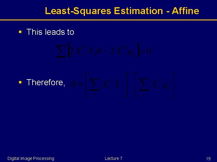
Least-Squares Estimation - Affine § This leads to § Therefore, Digital Image Processing Lecture 7 15

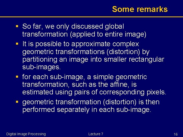
Some remarks § So far, we only discussed global transformation (applied to entire image) § It is possible to approximate complex geometric transformations (distortion) by partitioning an image into smaller rectangular sub-images. § for each sub-image, a simple geometric transformation, such as the affine, is estimated using pairs of corresponding pixels. § geometric transformation (distortion) is then performed separately in each sub-image. Digital Image Processing Lecture 7 16

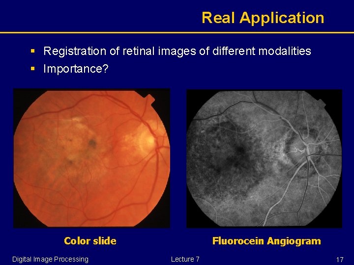
Real Application § Registration of retinal images of different modalities § Importance? Color slide Digital Image Processing Fluorocein Angiogram Lecture 7 17

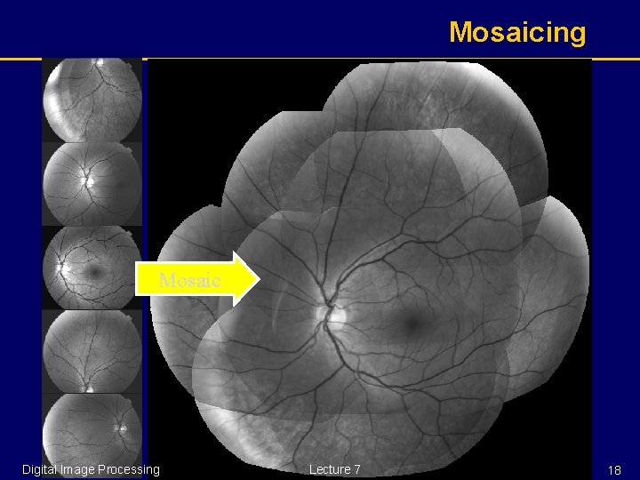
Mosaicing Mosaic Digital Image Processing Lecture 7 18

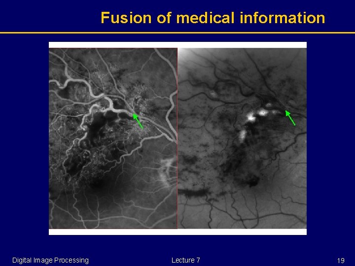
Fusion of medical information Digital Image Processing Lecture 7 19

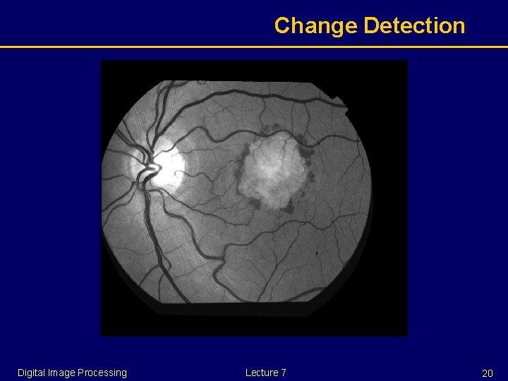
Change Detection Digital Image Processing Lecture 7 20

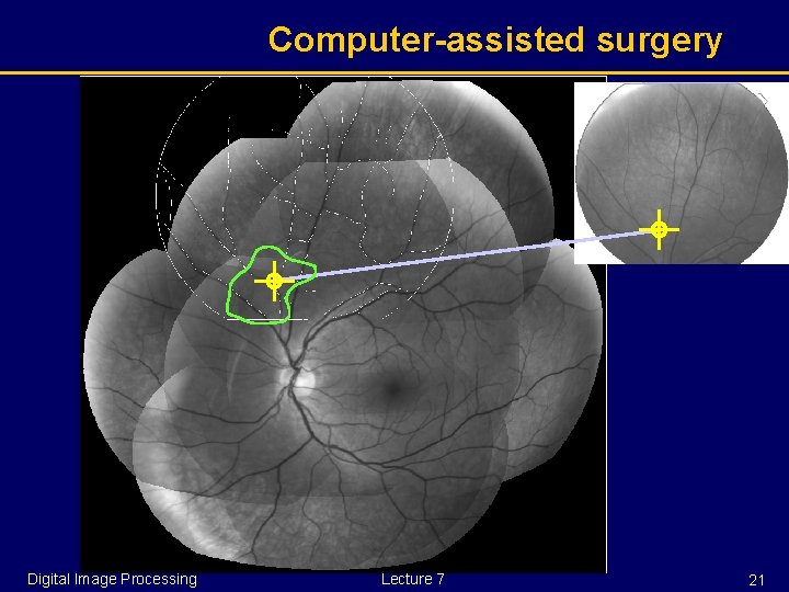
Computer-assisted surgery Digital Image Processing Lecture 7 21

What is needed? § A known transformation, which is less likely OR § Computing the transformation from features. § Feature extraction § Features in correspondence § Transformation models § Objective function Digital Image Processing Lecture 7 22

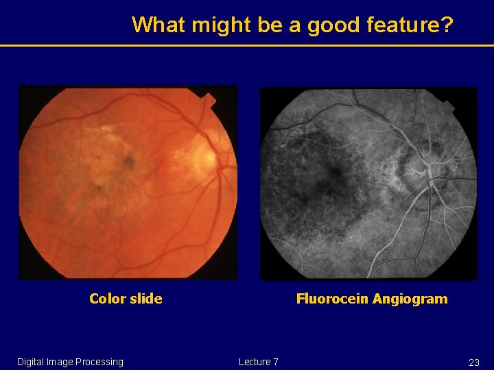
What might be a good feature? Color slide Digital Image Processing Fluorocein Angiogram Lecture 7 23

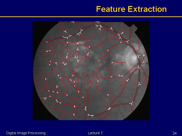
Feature Extraction Digital Image Processing Lecture 7 24

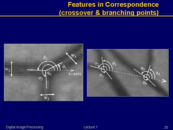
Features in Correspondence (crossover & branching points) Digital Image Processing Lecture 7 25

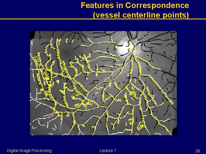
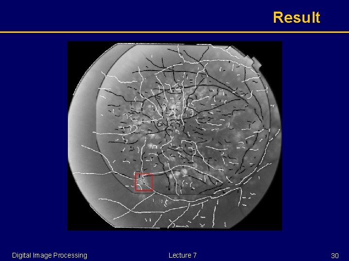
Features in Correspondence (vessel centerline points) Digital Image Processing Lecture 7 26

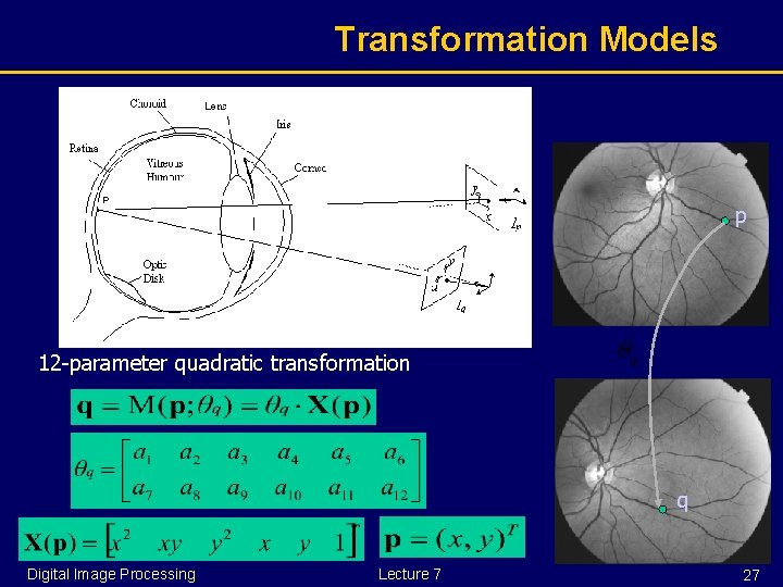
Transformation Models p 12 -parameter quadratic transformation q Digital Image Processing Lecture 7 27

Transformation Model Hierarchy Similarity Affine Reduced Quadratic Digital Image Processing Lecture 7 28

Objective Function Transformation parameters Feature point in image Set of correspondences Feature point in image Mapping of features from Digital Image Processing to based on Lecture 7 29

Result Digital Image Processing Lecture 7 30