Digital Image Processing Lecture 9 Intensity Graylevel Transformation

Digital Image Processing Lecture 9: Intensity (Gray-level) Transformation Functions using MATLAB

Function imadjust • Function imadjust is the basic IPT tool for intensity transformations of gray-scale images. It has the syntax: g = imadjust (f, [low_in high_in], [low_out high_out], gamma)

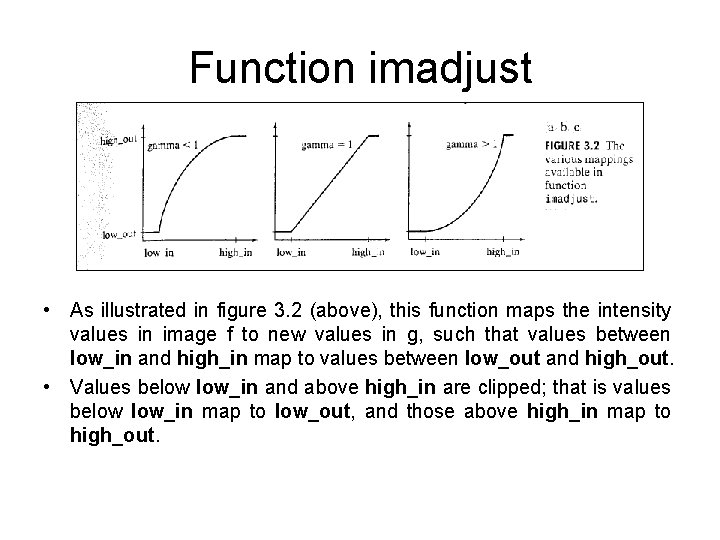
Function imadjust • As illustrated in figure 3. 2 (above), this function maps the intensity values in image f to new values in g, such that values between low_in and high_in map to values between low_out and high_out. • Values below low_in and above high_in are clipped; that is values below low_in map to low_out, and those above high_in map to high_out.

Function imadjust • The input image can be of class uint 8, uint 16, or double, and the output image has the same class as the input. • All inputs to function imadjust, other than f, are specified as values between 0 and 1, regardless of the class of f. If f is of class uint 8, imadjust multiplies the value supplied by 255 to determine the actual values to use; if f is of class uint 16, the values are multiplied by 65535. • Using the empty matrix ([ ]) for [low_in high_in] of for [low_out high_out] results in the default values [0 1]. • If high_out is less than low_out, the output intensity is reversed.

Function imadjust • Parameter gamma specifies the shape of the curve that maps the intensity values of f to create g. If gamma is less than 1, the mapping is weighted toward higher (brighter) output values, as fig 3. 2 (a) shows. If gamma is greater than 1, the mapping is weighted toward lower (darker) output values. If it is omitted from the function arguments, gamma defaults to 1 (linear mapping).

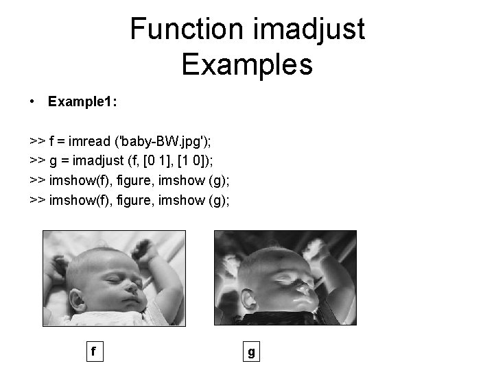
Function imadjust Examples • Example 1: >> f = imread ('baby-BW. jpg'); >> g = imadjust (f, [0 1], [1 0]); >> imshow(f), figure, imshow (g); f g

Function imadjust Examples • Cont. Example 1: This process, which is the digital equivalent of obtaining a photographic negative, is particularly useful for enhancing white or gray detail embedded in a large dark region. The negative of an image can be obtained also with IPT function imcomplement: g = imcomplement (f);

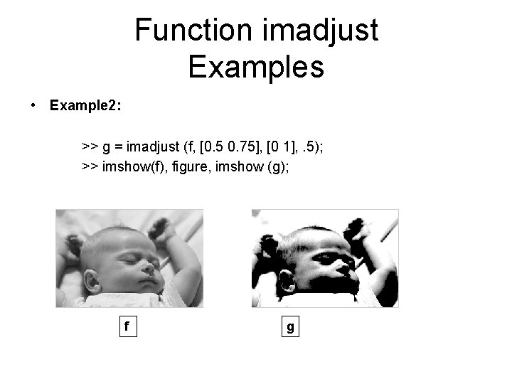
Function imadjust Examples • Example 2: >> g = imadjust (f, [0. 5 0. 75], [0 1], . 5); >> imshow(f), figure, imshow (g); f g

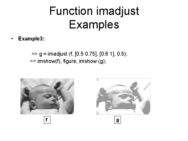
Function imadjust Examples • Example 3: >> g = imadjust (f, [0. 5 0. 75], [0. 6 1], 0. 5); >> imshow(f), figure, imshow (g); f g

Function imadjust Examples • Example 4: >> g = imadjust (f, [ ], 2); >> imshow(f), figure, imshow (g); f g

Logarithmic Transformations • The shape of logarithmic function curve, is similar to the gamma curve where gamma < 1, where low values set to 0 and high values set to 1 on both scales. • The shape of the gamma curve is variable (because of the change of low and high values), while the shape of the log function is fixed. • Logarithmic transformations are implemented using the expression: g = c * log (1 + double (f))

Logarithmic Transformations • But this function changes the data class of the image to double, so another sentence to return it back to uint 8 should be done: gs = im 2 uint 8 (mat 2 gray(g)); • Use of mat 2 gray brings the values to the range [0 1] and im 2 uint 8 brings them to the range [0 255]

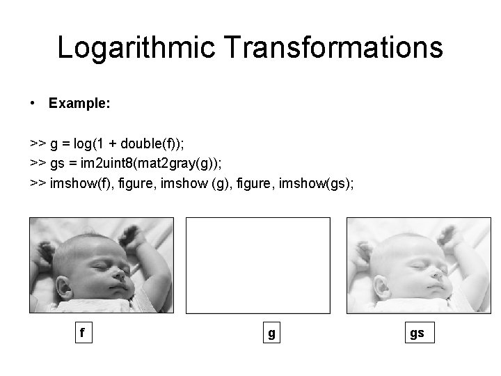
Logarithmic Transformations • Example: >> g = log(1 + double(f)); >> gs = im 2 uint 8(mat 2 gray(g)); >> imshow(f), figure, imshow (g), figure, imshow(gs); f g gs

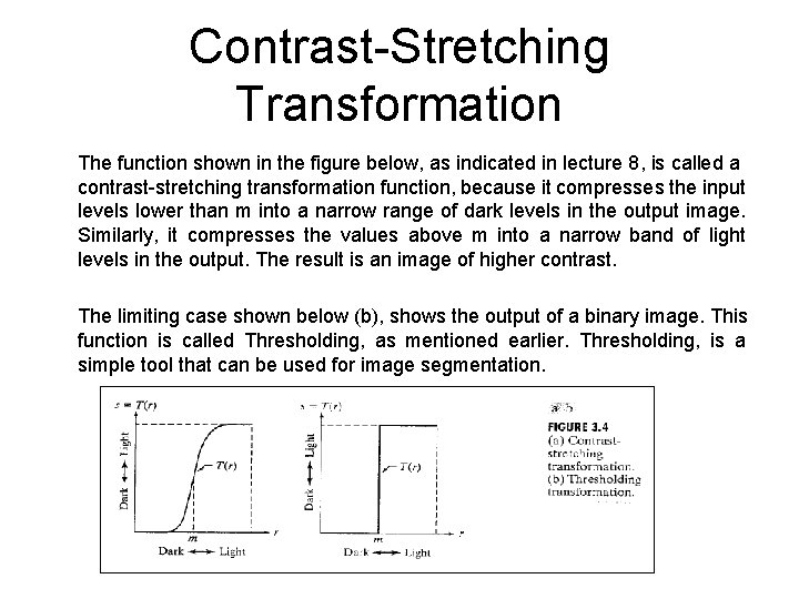
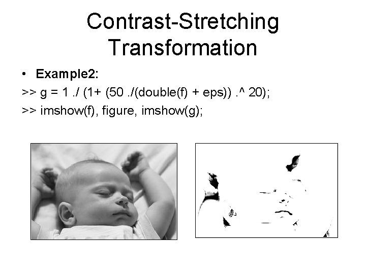
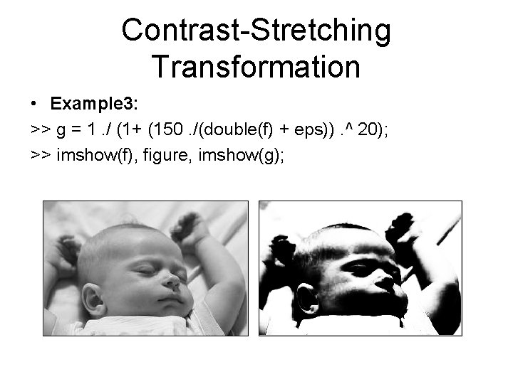
Contrast-Stretching Transformation The function shown in the figure below, as indicated in lecture 8, is called a contrast-stretching transformation function, because it compresses the input levels lower than m into a narrow range of dark levels in the output image. Similarly, it compresses the values above m into a narrow band of light levels in the output. The result is an image of higher contrast. The limiting case shown below (b), shows the output of a binary image. This function is called Thresholding, as mentioned earlier. Thresholding, is a simple tool that can be used for image segmentation.

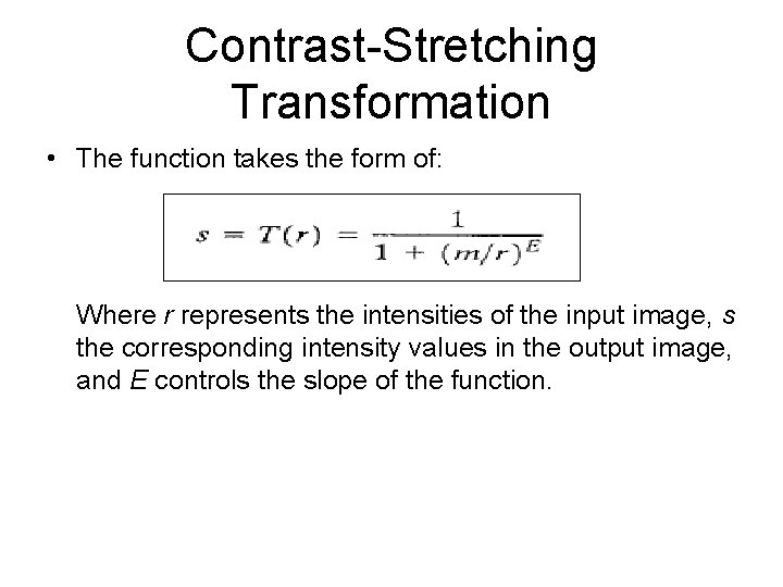
Contrast-Stretching Transformation • The function takes the form of: Where r represents the intensities of the input image, s the corresponding intensity values in the output image, and E controls the slope of the function.

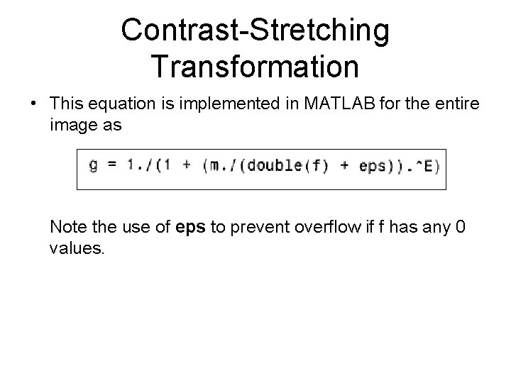
Contrast-Stretching Transformation • This equation is implemented in MATLAB for the entire image as Note the use of eps to prevent overflow if f has any 0 values.

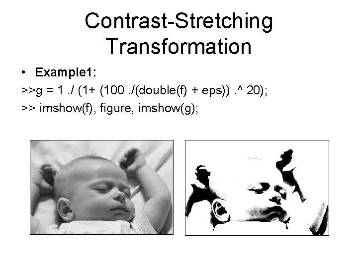
Contrast-Stretching Transformation • Example 1: >>g = 1. / (1+ (100. /(double(f) + eps)). ^ 20); >> imshow(f), figure, imshow(g);

Contrast-Stretching Transformation • Example 2: >> g = 1. / (1+ (50. /(double(f) + eps)). ^ 20); >> imshow(f), figure, imshow(g);

Contrast-Stretching Transformation • Example 3: >> g = 1. / (1+ (150. /(double(f) + eps)). ^ 20); >> imshow(f), figure, imshow(g);