Image Processing Chapter3 Part 3 Intensity Transformation and

Image Processing Chapter(3) Part 3: Intensity Transformation and spatial filters Prepared by: Hanan Hardan

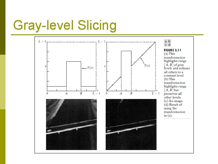
Gray-level Slicing p This technique is used to highlight a specific range of gray levels in a given image. – Similar to thresholding – Other levels can be suppressed or maintained – Useful for highlighting features in an image p It can be implemented in several ways, but the two basic themes are: n One approach is to display a high value for all gray levels in the range of interest and a low value for all other gray levels. n The second approach, based on the transformation brightens the desired range of gray levels but preserves gray levels unchanged.

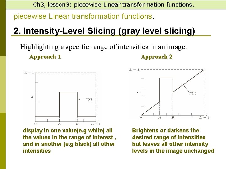
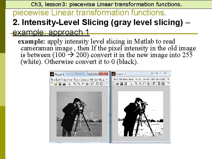
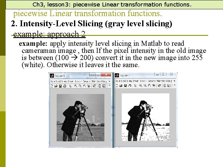
Ch 3, lesson 3: piecewise Linear transformation functions. 2. Intensity-Level Slicing (gray level slicing) Highlighting a specific range of intensities in an image. Approach 1 display in one value(e. g white) all the values in the range of interest , and in another (e. g black) all other intensities Approach 2 Brightens or darkens the desired range of intensities but leaves all other intensity levels in the image unchanged

Gray-level Slicing

Ch 3, lesson 3: piecewise Linear transformation functions. 2. Intensity-Level Slicing (gray level slicing) – example: approach 1 example: apply intensity level slicing in Matlab to read cameraman image , then If the pixel intensity in the old image is between (100 200) convert it in the new image into 255 (white). Otherwise convert it to 0 (black).

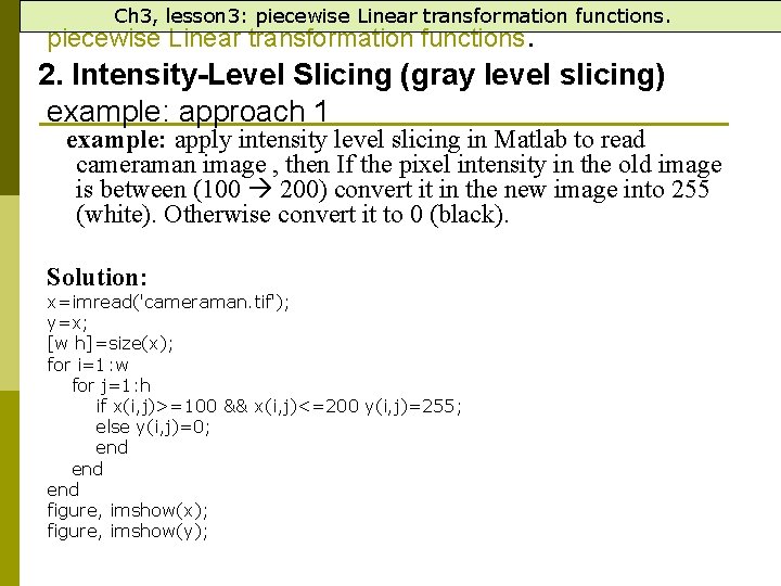
Ch 3, lesson 3: piecewise Linear transformation functions. 2. Intensity-Level Slicing (gray level slicing) example: approach 1 example: apply intensity level slicing in Matlab to read cameraman image , then If the pixel intensity in the old image is between (100 200) convert it in the new image into 255 (white). Otherwise convert it to 0 (black). Solution: x=imread('cameraman. tif'); y=x; [w h]=size(x); for i=1: w for j=1: h if x(i, j)>=100 && x(i, j)<=200 y(i, j)=255; else y(i, j)=0; end end figure, imshow(x); figure, imshow(y);

Ch 3, lesson 3: piecewise Linear transformation functions. 2. Intensity-Level Slicing (gray level slicing) example: approach 2 example: apply intensity level slicing in Matlab to read cameraman image , then If the pixel intensity in the old image is between (100 200) convert it in the new image into 255 (white). Otherwise it leaves it the same.

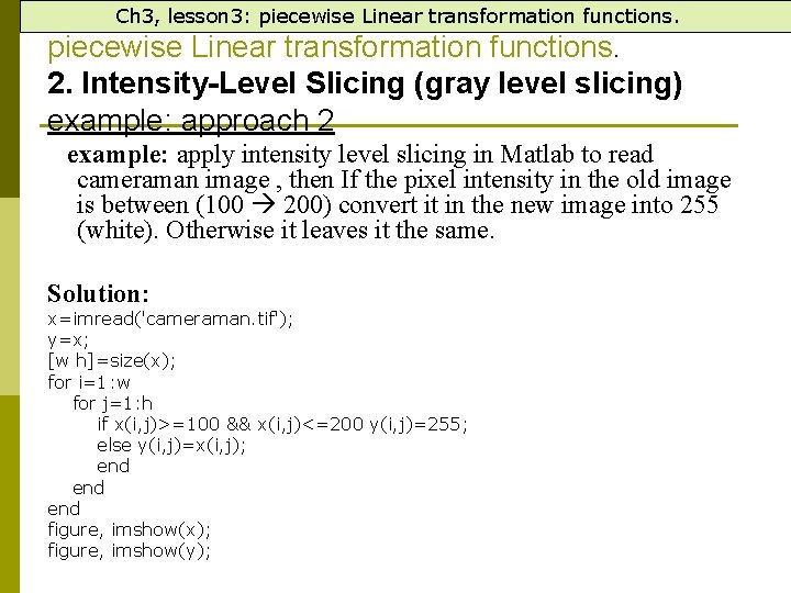
Ch 3, lesson 3: piecewise Linear transformation functions. 2. Intensity-Level Slicing (gray level slicing) example: approach 2 example: apply intensity level slicing in Matlab to read cameraman image , then If the pixel intensity in the old image is between (100 200) convert it in the new image into 255 (white). Otherwise it leaves it the same. Solution: x=imread('cameraman. tif'); y=x; [w h]=size(x); for i=1: w for j=1: h if x(i, j)>=100 && x(i, j)<=200 y(i, j)=255; else y(i, j)=x(i, j); end end figure, imshow(x); figure, imshow(y);

Ch 3, lesson 3: piecewise Linear transformation functions. 2. Intensity-Level Slicing (gray level slicing) Homework example: apply intensity level slicing (approch 2) in Matlab to read moon image , then If the pixel intensity in the old image is between (0 20) convert it in the new image into 130.

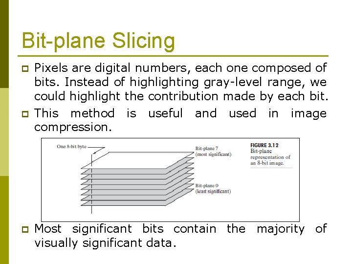
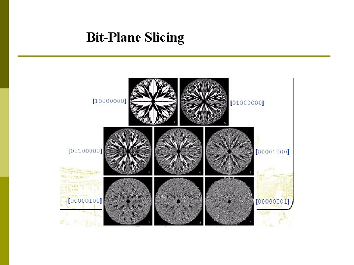
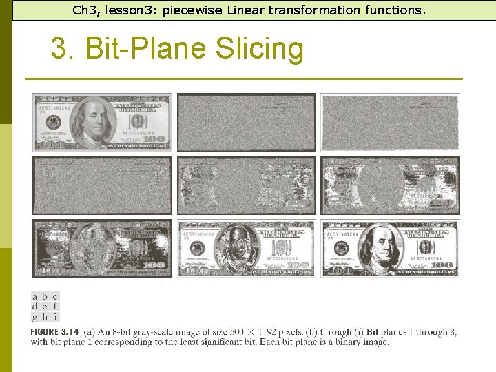
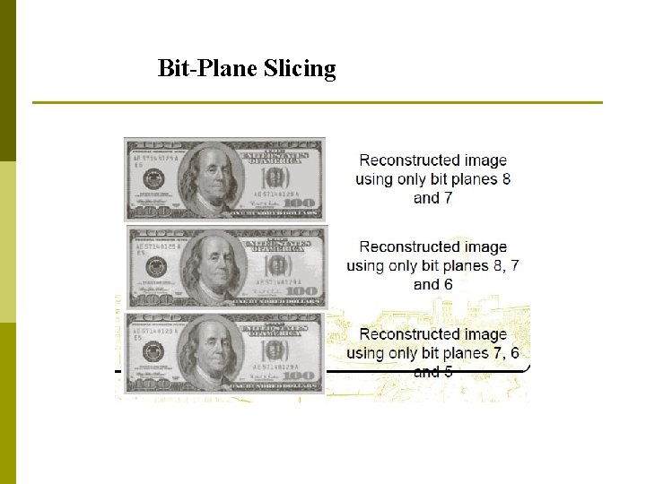
Bit-plane Slicing p p p Pixels are digital numbers, each one composed of bits. Instead of highlighting gray-level range, we could highlight the contribution made by each bit. This method is useful and used in image compression. Most significant bits contain the majority of visually significant data.

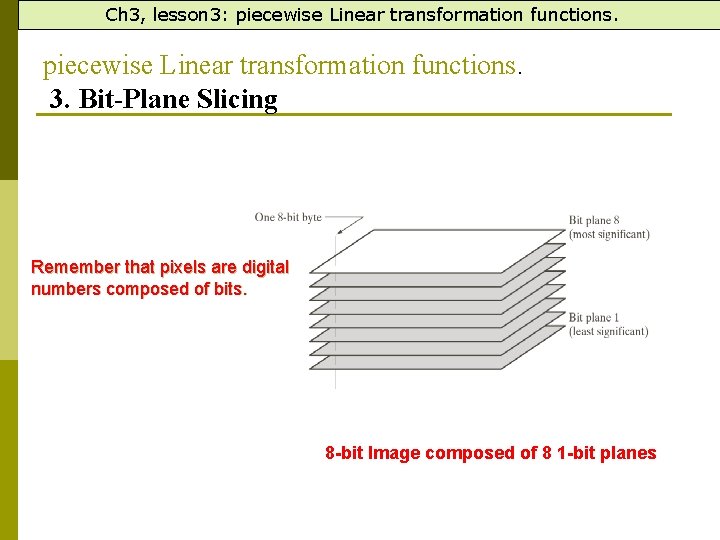
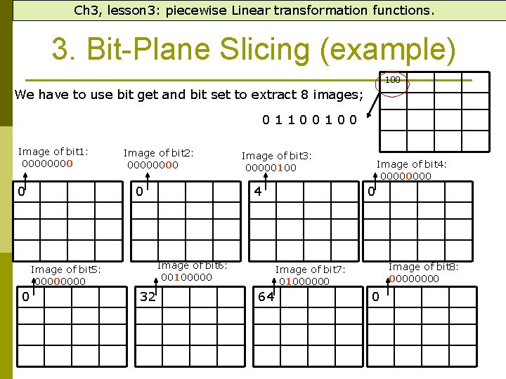
Ch 3, lesson 3: piecewise Linear transformation functions. 3. Bit-Plane Slicing Remember that pixels are digital numbers composed of bits. 8 -bit Image composed of 8 1 -bit planes

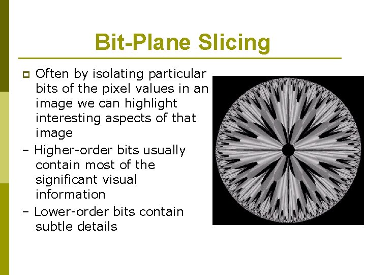
Bit-Plane Slicing Often by isolating particular bits of the pixel values in an image we can highlight interesting aspects of that image – Higher-order bits usually contain most of the significant visual information – Lower-order bits contain subtle details p

Bit-Plane Slicing

Ch 3, lesson 3: piecewise Linear transformation functions. 3. Bit-Plane Slicing

Bit-Plane Slicing

Ch 3, lesson 3: piecewise Linear transformation functions. 3. Bit-Plane Slicing (example) 100 We have to use bit get and bit set to extract 8 images; 01100100 Image of bit 1: 0000 0 Image of bit 2: 0000 0 4 Image of bit 6: 00100000 Image of bit 5: 0000 0 Image of bit 3: 00000100 32 Image of bit 4: 0000 0 Image of bit 8: 0000 Image of bit 7: 01000000 64 0

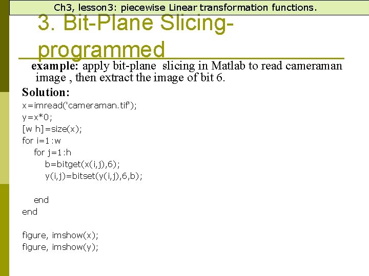
Ch 3, lesson 3: piecewise Linear transformation functions. 3. Bit-Plane Slicingprogrammed example: apply bit-plane slicing in Matlab to read cameraman image , then extract the image of bit 6. Solution: x=imread('cameraman. tif'); y=x*0; [w h]=size(x); for i=1: w for j=1: h b=bitget(x(i, j), 6); y(i, j)=bitset(y(i, j), 6, b); end figure, imshow(x); figure, imshow(y);

Histogram Processing What is a Histogram? p In Statistics, Histogram is a graphical representation showing a visual impression of the distribution of data. p An Image Histogram is a type of histogram that acts as a graphical representation of the lightness/color distribution in a digital image. It plots the number of pixels for each value.

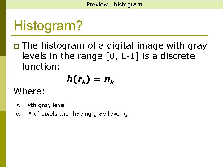
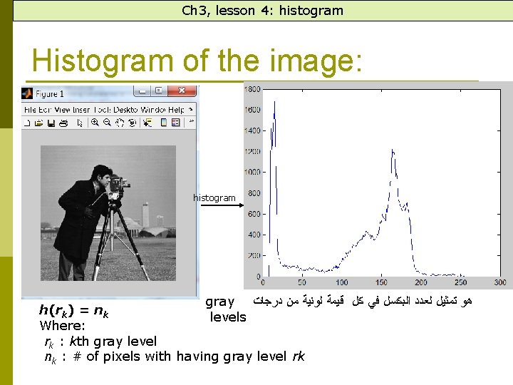
Preview. . histogram Histogram? The histogram of a digital image with gray levels in the range [0, L-1] is a discrete function: h(rk) = nk Where: p rk : kth gray level nk : # of pixels with having gray level rk

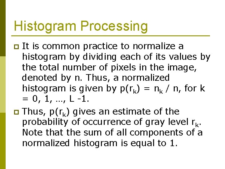
Histogram Processing It is common practice to normalize a histogram by dividing each of its values by the total number of pixels in the image, denoted by n. Thus, a normalized histogram is given by p(rk) = nk / n, for k = 0, 1, …, L -1. p Thus, p(rk) gives an estimate of the probability of occurrence of gray level rk. Note that the sum of all components of a normalized histogram is equal to 1. p

? Why Histograms are the basis for numerous spatial domain processing techniques p Histogram manipulation can be used effectively for image enhancement p Histograms can be used to provide useful image statistics p Information derived from histograms are quite useful in other image processing applications, such as image compression and segmentation. p

Ch 3, lesson 4: histogram Histogram of the image: histogram gray ﻫﻮ ﺗﻤﺜﻴﻞ ﻟﻌﺪﺩ ﺍﻟﺒﻜﺴﻞ ﻓﻲ ﻛﻞ ﻗﻴﻤﺔ ﻟﻮﻧﻴﺔ ﻣﻦ ﺩﺭﺟﺎﺕ h ( rk ) = n k levels Where: rk : kth gray level nk : # of pixels with having gray level rk

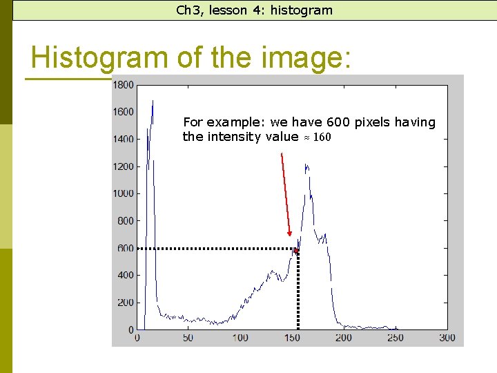
Ch 3, lesson 4: histogram Histogram of the image: For example: we have 600 pixels having the intensity value ≈ 160

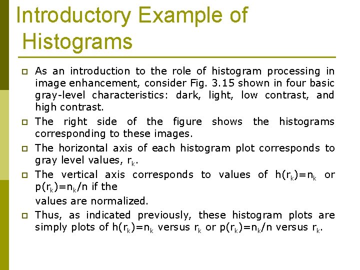
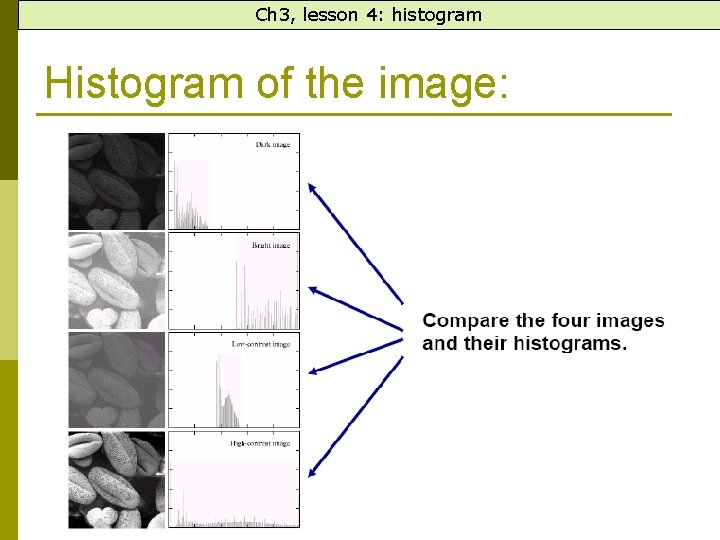
Introductory Example of Histograms p p p As an introduction to the role of histogram processing in image enhancement, consider Fig. 3. 15 shown in four basic gray-level characteristics: dark, light, low contrast, and high contrast. The right side of the figure shows the histograms corresponding to these images. The horizontal axis of each histogram plot corresponds to gray level values, rk. The vertical axis corresponds to values of h(rk)=nk or p(rk)=nk/n if the values are normalized. Thus, as indicated previously, these histogram plots are simply plots of h(rk)=nk versus rk or p(rk)=nk/n versus rk.

Ch 3, lesson 4: histogram Histogram of the image:

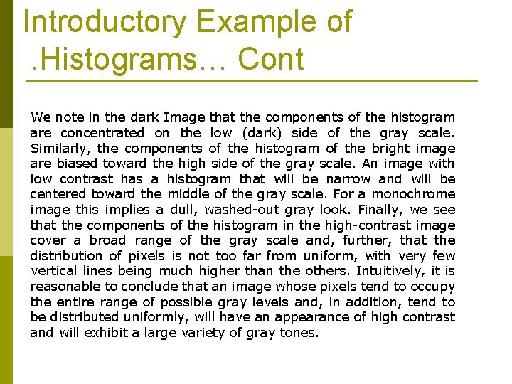
Introductory Example of. Histograms… Cont We note in the dark Image that the components of the histogram are concentrated on the low (dark) side of the gray scale. Similarly, the components of the histogram of the bright image are biased toward the high side of the gray scale. An image with low contrast has a histogram that will be narrow and will be centered toward the middle of the gray scale. For a monochrome image this implies a dull, washed-out gray look. Finally, we see that the components of the histogram in the high-contrast image cover a broad range of the gray scale and, further, that the distribution of pixels is not too far from uniform, with very few vertical lines being much higher than the others. Intuitively, it is reasonable to conclude that an image whose pixels tend to occupy the entire range of possible gray levels and, in addition, tend to be distributed uniformly, will have an appearance of high contrast and will exhibit a large variety of gray tones.

Histogram in MATLAB h = imhist (f, b) Where f, is the input image, h is the histogram, b is number of bins (tick marks) used in forming the histogram (b = 255 is the default) A bin, is simply, a subdivision of the intensity scale. For example, if we are working with uint 8 images and we let b = 2, then the intensity scale is subdivided into two ranges: 0 – 127 and 128 – 255. the resulting histograms will have two values: h(1) equals to the number of pixels in the image with values in the interval [0, 127], and h(2) equal to the number of pixels with values in the interval [128 255].

Histogram in MATLAB p We obtain the normalized histogram simply by using the expression. p = imhist (f, b) / numel(f) numel (f): a MATLAB function that gives the number of elements in array f (i. e. the number of pixels in an image.

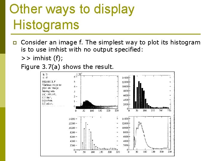
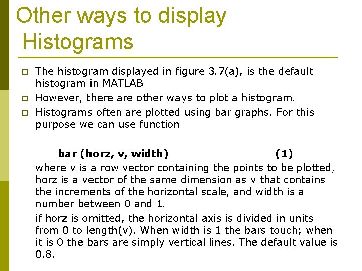
Other ways to display Histograms p Consider an image f. The simplest way to plot its histogram is to use imhist with no output specified: >> imhist (f); Figure 3. 7(a) shows the result.

Other ways to display Histograms p p p The histogram displayed in figure 3. 7(a), is the default histogram in MATLAB However, there are other ways to plot a histogram. Histograms often are plotted using bar graphs. For this purpose we can use function bar (horz, v, width) (1) where v is a row vector containing the points to be plotted, horz is a vector of the same dimension as v that contains the increments of the horizontal scale, and width is a number between 0 and 1. if horz is omitted, the horizontal axis is divided in units from 0 to length(v). When width is 1 the bars touch; when it is 0 the bars are simply vertical lines. The default value is 0. 8.

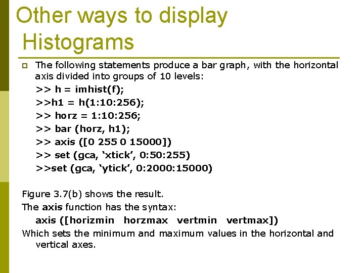
Other ways to display Histograms p The following statements produce a bar graph, with the horizontal axis divided into groups of 10 levels: >> h = imhist(f); >>h 1 = h(1: 10: 256); >> horz = 1: 10: 256; >> bar (horz, h 1); >> axis ([0 255 0 15000]) >> set (gca, ‘xtick’, 0: 50: 255) >>set (gca, ‘ytick’, 0: 2000: 15000) Figure 3. 7(b) shows the result. The axis function has the syntax: axis ([horizmin horzmax vertmin vertmax]) Which sets the minimum and maximum values in the horizontal and vertical axes.

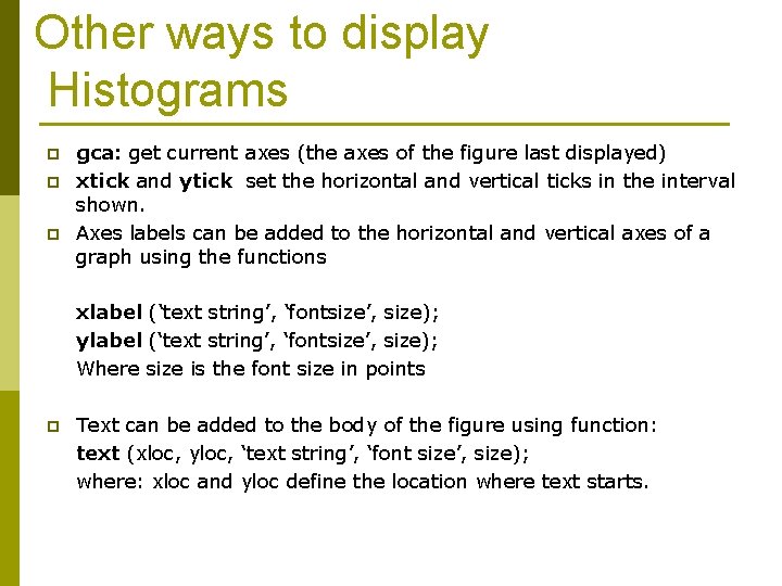
Other ways to display Histograms p p p gca: get current axes (the axes of the figure last displayed) xtick and ytick set the horizontal and vertical ticks in the interval shown. Axes labels can be added to the horizontal and vertical axes of a graph using the functions xlabel (‘text string’, ‘fontsize’, size); ylabel (‘text string’, ‘fontsize’, size); Where size is the font size in points p Text can be added to the body of the figure using function: text (xloc, yloc, ‘text string’, ‘font size’, size); where: xloc and yloc define the location where text starts.

Other ways to display Histograms p Note: functions that set axis values and labels are used after the function has been plotted. p A title can be added to a plot using: title(‘text string’)

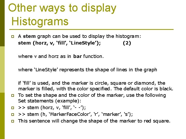
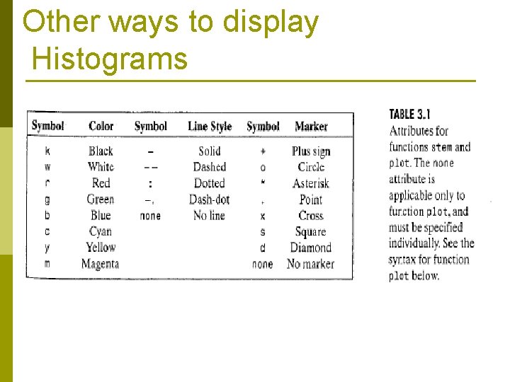
Other ways to display Histograms p A stem graph can be used to display the histogram: stem (horz, v, ‘fill’, ‘Line. Style’); (2) where v and horz as in bar function. where ‘Line. Style’ represents the shape of lines in the graph p p if ‘fill’ is used, and the marker is circle, square or diamond, the marker is filled, with the color specified. The default color is black. To set the shape and the color of the marker, use the following Set statements (example): >> stem (horz, v, ‘fill’, ‘- -’); >> stem (h, ‘Marker. Face. Color’, ‘marker’, ‘s’); This sentence will change the shape of the marker to red square.

Other ways to display Histograms

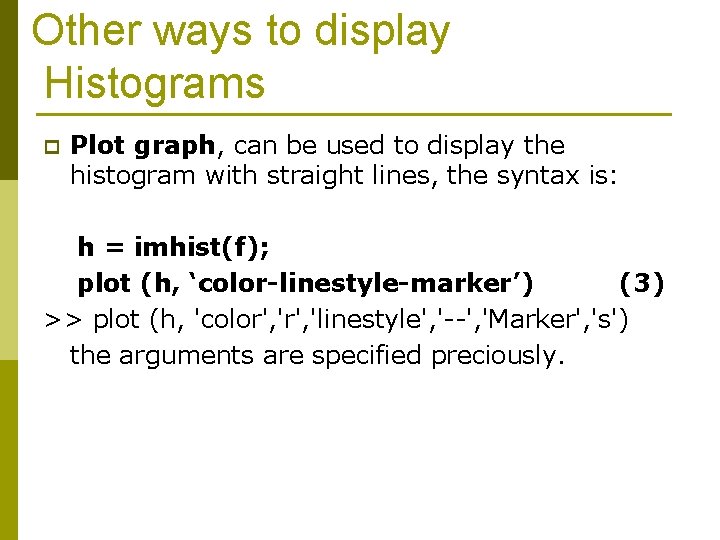
Other ways to display Histograms p Plot graph, can be used to display the histogram with straight lines, the syntax is: h = imhist(f); plot (h, ‘color-linestyle-marker’) (3) >> plot (h, 'color', 'linestyle', '--', 'Marker', 's') the arguments are specified preciously.

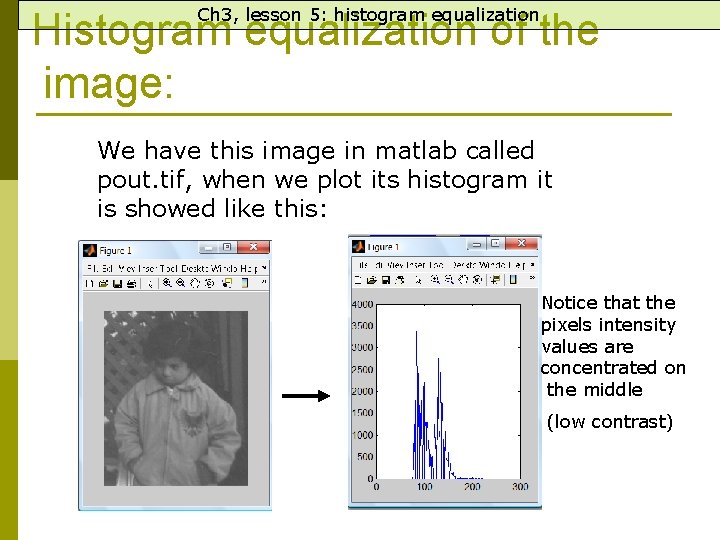
Ch 3, lesson 5: histogram equalization Histogram equalization of the image: We have this image in matlab called pout. tif, when we plot its histogram it is showed like this: Notice that the pixels intensity values are concentrated on the middle (low contrast)

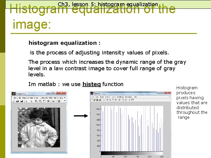
Ch 3, lesson 5: histogram equalization Histogram equalization of the image: histogram equalization : is the process of adjusting intensity values of pixels. The process which increases the dynamic range of the gray level in a law contrast image to cover full range of gray levels. Im matlab : we use histeq function Histogram produces pixels having values that are distributed throughout the range

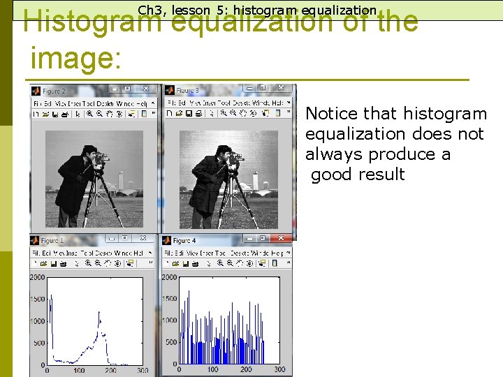
Ch 3, lesson 5: histogram equalization Histogram equalization of the image: Notice that histogram equalization does not always produce a good result

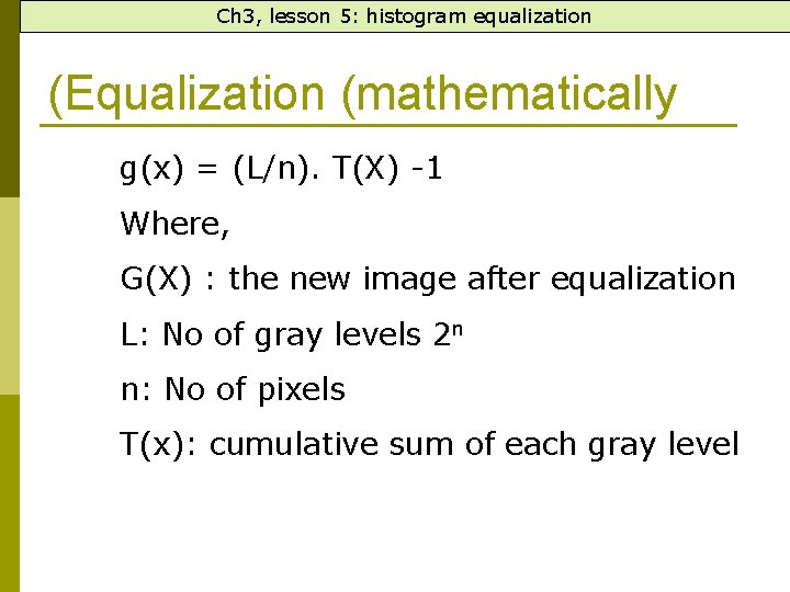
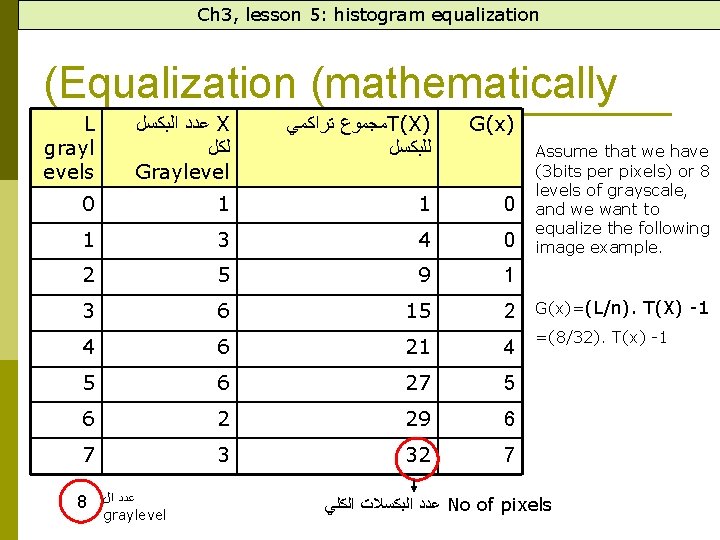
Ch 3, lesson 5: histogram equalization (Equalization (mathematically g(x) = (L/n). T(X) -1 Where, G(X) : the new image after equalization L: No of gray levels 2 n n: No of pixels T(x): cumulative sum of each gray level

Ch 3, lesson 5: histogram equalization (Equalization (mathematically L grayl evels ﻋﺪﺩ ﺍﻟﺒﻜﺴﻞ X ﻟﻜﻞ Graylevel ﻣﺠﻤﻮﻉ ﺗﺮﺍﻛﻤﻲ T(X) ﻟﻠﺒﻜﺴﻞ G(x) 0 1 1 0 1 3 4 0 2 5 9 1 3 6 15 2 4 6 21 4 5 6 27 5 6 2 29 6 7 3 32 7 8 ﻋﺪﺩ ﺍﻝ graylevel Assume that we have (3 bits per pixels) or 8 levels of grayscale, and we want to equalize the following image example. G(x)=(L/n). T(X) -1 =(8/32). T(x) -1 ﻋﺪﺩ ﺍﻟﺒﻜﺴﻼﺕ ﺍﻟﻜﻠﻲ No of pixels