Digital Image Processing Image Transformation Dr Ji Zhen

数字图像处理 Digital Image Processing 图像变换 Image Transformation 纪震博士Dr. Ji Zhen Faculty of Information Engineering, SZU 2003. 01 1

Basic Concepts v Image information can be transformed into different spaces by different transforms; T : X Y X is source space Y is object space § Reversible § Computation is simple in Transformed space § Transform algorithm is simple Dr. JI ZHEN 2

Properties of Image Transforms a) b) c) Simplify algorithm. For example q Convolution in spatial space —— Multiplication in frequency space Some characteristics of image can be recognized easily in transformed space. For example q In Transformed space, image energy can be more concentrated, which can be used to compress the image. Several transformation can be used to extract features of images. For example： q K-L Transformation Dr. JI ZHEN 3

Contents of Image Transformation § § § § Basis Images The Discrete Fourier Transform (DFT) The Discrete Cosine Transform (DCT) The Hadamard-Walsh Transform The Haar Transform The Karhumen-Loeve Transform The Discrete Wavelet Transform (DWT) Dr. JI ZHEN 4

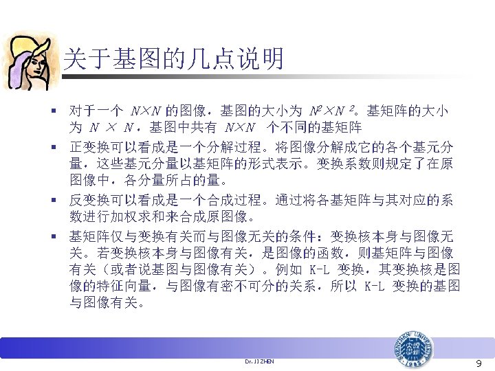
Basis Images (基图) § The inverse tow-dimensional transform can be viewed as reconstructing the image by summing a set of properly weighted basis images. § A basis image can be generated by inverse transforming a coefficient matrix containing only one nonzero element, which is set to unity. § Image transform can be written as： [F(u, v)]=A [ f (x, y)] BT [ f (u, v)]=A [F(x, y)] BT Where ，AT=[a 1, a 2, …, a. N]， BT=[b 1, b 2, …, b. N]， ai, bi is N× 1 vector Dr. JI ZHEN 5

Basis Images Then is a N×N matrix Dr. JI ZHEN 6

Basis Images § The basis images can be thought of as a set of basic components into which any image can be decomposed. They are also the building blocks from which any image can be reassembled. § The forward transform does the decomposition by determining the coefficients. § The inverse transform does the reconstitution by summing the basis images, weighted by those coefficients aij. Dr. JI ZHEN 7

Basis Matrix, Basis Image § Basis matrix is the matrix [aibj. T]N × N § basis image is a matrix defined as Dr. JI ZHEN 8

Discrete Fourier Transform (DFT) § Image f(x, y), 0≤x≤M-1, 0≤y≤N-1 § Transform kernel § Discrete Fourier Transform of f(x, y)is Dr. JI ZHEN 10

Discrete Fourier Transform (DFT) § In generally, M=N. Transform kernel can be represented as: § Discrete Fourier Transform of f(x, y) can be represented as Dr. JI ZHEN 11

Modulus、Phase、Power Spectrum Let R(u, v)、I(u, v) be real part and imaginary part of F(u, v) Modulus： Phase： Power Spectrum： Dr. JI ZHEN 12

Basis Matrix of The Fourier Transform § The Fourier Transform：A=B=AT=BT=W where § Basis Matrix Dr. JI ZHEN 13

Basis Images of The Fourier Transform (N=8 Phase Image) Dr. JI ZHEN 14

Transform (Example) img=imread('lena. bmp', 'bmp'); subplot(121); imshow(img); title('original image ') fimg=fftshift(fft 2(img)); subplot(122); imshow(abs(fimg)/10000) title(' transformed image ') Dr. JI ZHEN 15

Transform (Example) A=zeros(128) ; A(33: 33+63, 33: 33+63)=255*ones(64); %A=imread('lena. bmp', 'bmp'); m = fft 2(A); m = fftshift(m); subplot(2, 2, 1); imshow(A); title('Original Image'); subplot(2, 2, 3) mm = log(1+abs(m)); mm = mm/max(mm))*255; imshow(uint 8(mm)); title('Modulus'); Dr. JI ZHEN 16

Transform (Example) （cont. ） subplot(2, 2, 4) ma= angle(m); ma = (ma-min(ma)))/(max(ma)) - min(ma)) )*255; imshow(uint 8(ma)); title('Phase'); [i, j] = find(abs(m)==max(abs(m)))); m(i, j) = m(i, j)*2; s = ifft 2(m); subplot(2, 2, 2) imshow(uint 8(abs(s))); title('Reconstruction Image'); Dr. JI ZHEN 17

Transform (Example) Dr. JI ZHEN 18

Transform (Example) Dr. JI ZHEN 19

Properties of 2 -Dimensional Fourier Transform § § § § § 1. Separability 2. Linearity 3. Scality 4. Shift Theorem 5. Rotation 6. Periodicity and conjugation 7. Convolution 8. Correlation 9. Average Dr. JI ZHEN 20

1. Separability Transform kernel of 2 -Dimensional DFT is Separating the transformation into horizontal and vertical operations. At first, one-dimensional DFTs can be computed on the rows of the image. Next, performs columnwise one-dimensional DFTs on the resulting array. Dr. JI ZHEN 21

1. Separability n The implementation steps for the two-dimensional DFT may be visualised as shown in the diagram below f(x, y) Column Transforms F(x, v) Row Transforms F(u, v) Multiply by N Dr. JI ZHEN 22

1. Separability Dr. JI ZHEN 23

2. Linearity DFT is a linear operator a f 1(x, y)+b f 2(x, y) a. F 1(u, v)+b. F 2(u, v) Dr. JI ZHEN 24

3. Scality Dr. JI ZHEN 25

3. Scality Dr. JI ZHEN 26

4. Shift Theorem Dr. JI ZHEN 27

4. Shift Theorem In digital image processing, it is necessary to shift the origin of F(u, v) to the center of N×N frequency domain. Let：u 0=v 0=N/2，then Dr. JI ZHEN 28

4. Shift Theorem Dr. JI ZHEN 29

4. Shifting Sample（Frequency Shifting） Dr. JI ZHEN 30

5. Rotation In polar coordinates, f (x, y) and F(u, v) can be represented by f(r, θ) and F(w, φ) alternatively. Then f (r, θ+ θ 0) F(w，φ + θ 0) Dr. JI ZHEN 31

5. Rotation Sample Dr. JI ZHEN 32

6. Periodicity and conjugation Periodicity ： F(u, v) = F(u+a. N, v+b. N) f (x, y) = f (x+a. N, y+b. N) Where a, b = 0, ± 1, ± 2, …… Conjugation： F(u, v) = F*(-u, -v) |F(u, v)| = |F(-u, -v)| Dr. JI ZHEN 33

7. Convolution 2 -D convolution is defined as： Then：f(x，y)*g(x，y) F(u，v)G(u，v) f(x，y)g(x，y) F(u，v)*G(u，v) Dr. JI ZHEN 34

8. Correlation 2 -D correlation is defined as： Correlation Theorems： Dr. JI ZHEN 35

9. Average of 2 D image f (x, y) is defined as： Let u=v=0 , then: Dr. JI ZHEN 36

Discrete Cosine Transform（DCT） Transform kernel of two-dimensional DCT is where Clearly, the kernel for the DCT is both separable and symmetric, and hence the DCT may be implemented as a series of one dimensional DCTs. Dr. JI ZHEN 39

Discrete Cosine Transform（DCT） Forward transform and Inverse transform where u, v, x, y = 0, 1, 2, …, N-1 Dr. JI ZHEN 40

Discrete Cosine Transform（DCT） To enable an application of the concept of the DCY and its relation to the DFT discussed earlier, consider the modified basis function gdctmod(x, u) defined below As compared to the (unmodified) DFT basis function It can be seen that, neglecting the scaling factors, the modified DCT is similar in form to the real part of the DFT, but is not identical due to the extra 2 on the denominator of the cos argument. In fact we can see that the modified DCT would be identical (again neglecting the scaling factors) to the first half (i. e. from u=0 to N-1) of the real part of a DFT of size 2 N. Hence it can be seen, as stated earlier, that DCT analysis implies periodicity of period 2 N points (for a DCT analysis of an N-point signal). Dr. JI ZHEN 41

Transform Matrix of DCT where： Dr. JI ZHEN 42

Transform Matrix of DCT (N=8) Dr. JI ZHEN 43

Transform Matrix of DCT (N=8) N=8; u = zeros(N, N); u(1, 1: N) = 1. 0/sqrt(2. 0); for i=2: N for j=1: N u(i, j) = cos((2*j-1)*(i-1)*pi/(2. 0*N)); end u = sqrt(2. 0/N)*u; imagesc(u) colormap(gray); axis off Dr. JI ZHEN 44

Basis Images of DCT(N=8) Dr. JI ZHEN 45

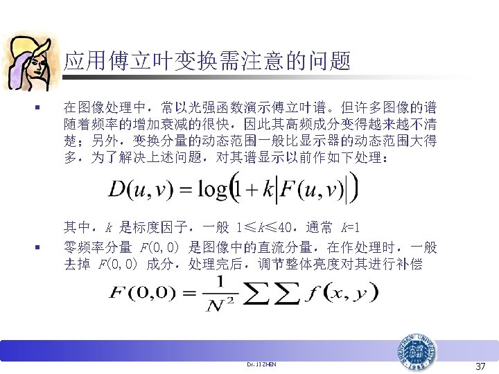
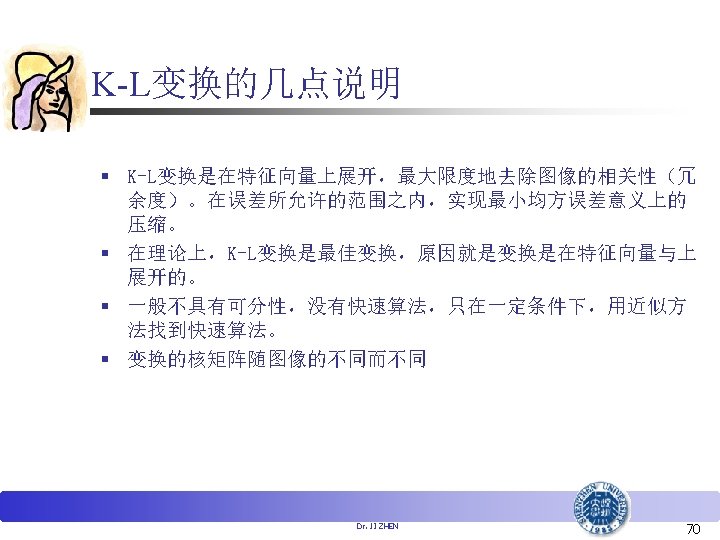
Example of DCT [a, map] = imread('lena. bmp', 'bmp'); subplot(1, 2, 1); J = dct 2(a); imshow(log(abs(J)), []); colormap(jet); J(abs(J)<50) = 0; K = idct 2(J); subplot(1, 2, 2); imshow(K, [0 255]); Dr. JI ZHEN 46

Example of DCT img=imread('lena. bmp', 'bmp'); subplot(121) imshow(img); title('original image') dcimg=dct 2(img); subplot(122) imshow(100*dcimg/dcimg(1, 1)); title('DCT coefficients') Dr. JI ZHEN 47

Example of DCT Dr. JI ZHEN 48

Example of DCT N = 8; I = imread('e: cameraman. bmp'); I = double(I)/255; N = 16; dctm = dctmtx(N); mask = ones(N, N); image. DCT = blkproc(I, [N N], 'P 1*x*P 2', dctm. '); th = max(image. DCT))/80; index = find(image. DCT<th); image. DCT(index) = 0; Dr. JI ZHEN 49

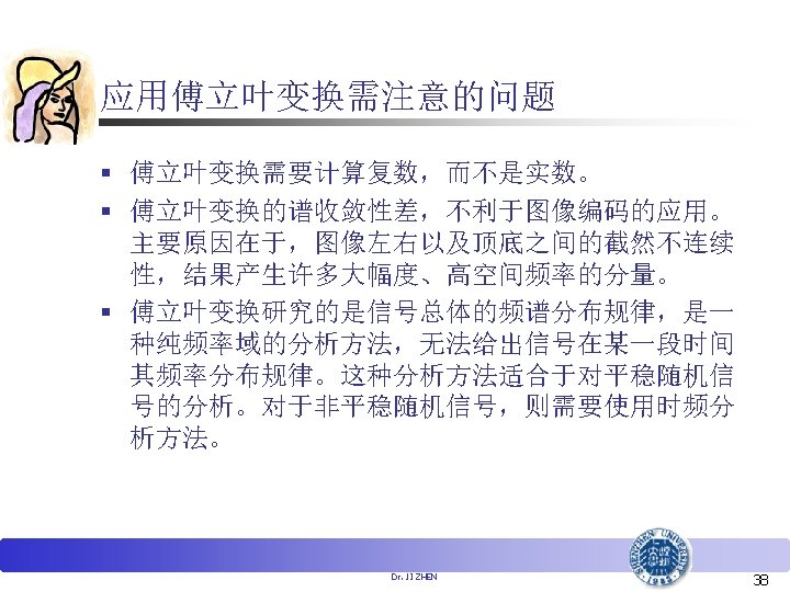
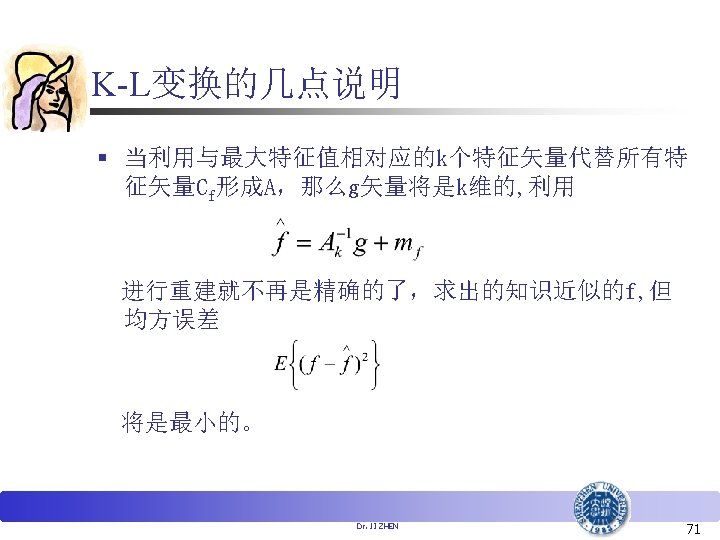
Example of DCT %cont. new. Image = blkproc(image. DCT, [N N], 'P 1*(x. *P 2)*P 3', dctm. ', mask(1: N, 1: N), dctm); index = find(new. Image>1); new. Image(index) = 1; index = find(new. Image<0); new. Image(index) = 0; figure; imshow(new. Image); Dr. JI ZHEN 50

Example of DCT Dr. JI ZHEN 51

Example of DCT dctdemo Dr. JI ZHEN 52

The Walsh-Hadamard Transform kernel of Two-Dimensional DWT Transform kernel of Two-Dimensional DHT Where bi(x) is the ith number of binary number x N = 2 n Dr. JI ZHEN 54

The Walsh-Hadamard Transform § The kernel matrix of DHT can be generated from the block matrix form § The sign change count is called sequency. § Reorder the rows to make sequency increase uniformly with row number. This yields a transform DWT § The sequency of DWT increases uniformly with row number, much as frequency increases with the Fourier kernel, which is somewhat easier to interpret. Dr. JI ZHEN 55

The Walsh Kernel matrix(N=8) Dr. JI ZHEN 56

The basis images of DWT(N=8) Dr. JI ZHEN 57

The Hadamard kernel matrix(N=8) Dr. JI ZHEN 58

The basis images of DHT(N=8) Dr. JI ZHEN 59

The Haar Transform § The Haar transform is a symmetric, separable unitary transformation that uses Haar funcitons for its basis. It exists for N=2 n, where n is an integer. § Whereas the Fourier transform basis functions differ only in frequency, the Haar functions vary in both scale(width) and position. This gives the Haar transform a dual scale-position nature that is evident in its basis functions. The Haar functions Dr. JI ZHEN 61

The kernel matrix for the Haar transform(N=4) Dr. JI ZHEN 62

The kernel matrix for the Haar transform(N=8) Dr. JI ZHEN 63

The Haar transform basis images(N=8) Dr. JI ZHEN 64

The K-L Transform(Hotelling) The K-L transform is variously called Hotelling transform, the eigenvector transform, or the method of principal componets. Suppose image set ：{ f 1(x, y), f 2(x, y), …, fi(x, y), …, f. L(x, y)} Where the correlation between fi(x, y) is commonly rather high. fi(x, y) can be represented as N 2 -by-1 vector Xi xij is the jth row of image fi(x, y). i=1, 2, …, L Dr. JI ZHEN 65

The K-L Transform The covariance matrix of vector X is defined as, Cf = E{(X-mf)T} The mean vector mf is mf =E{X} mf is N 2 -by-1 vector, Cf is N 2×N 2 matrix. In generally, mf and Cf can be represented approximately as, Dr. JI ZHEN 66

The K-L Transform Let ei and i be the eigenvectors and eigenvalues of Cf. Where i=1, 2, …, N 2, Suppose The K-L transform is g = A(X-mf) Dr. JI ZHEN 67

The Properties of the K-L transform § A)The mean vector of g, mg=0 mg =E{g}=E{A(X-mg)}=A E{X}-A mg=0 § B) The covariance matrix of g, Cg=A Cf AT Cg = E{(Y-mg)T} = E{gg. T} = E{(AX-Amg)T} = E{A(X-mg)TAT} = AE{(X-mg)T} AT = A Cf A T Dr. JI ZHEN 68

The Properties of the K-L transform § C)Cg is a diagonal matrix having the eigenvalues of Cg along its diagonal. The elements of g are uncorrelated. § D) The K-L transform is invertible. The original image can be reconstructed by A-1 = AT f = A-1 f + mf Dr. JI ZHEN 69