Image Processing Digital Image Processing Teacher Assistant Elhanan

Image Processing Digital Image Processing • Teacher Assistant: Elhanan Elboher course email : impr@cs. huji. ac. il personal email : elhanan. elboher@mail. huji. ac. il • Reception hour: Thursday 14: 00 -15: 00 • Web site: www. cs. huji. ac. il/~impr 1

Image Processing Administration • All exercises are mandatory • 3 Exams and Moed B • Please register online asap! 2

Image Processing Today Outline • Matlab Basics • Intensity transform and Histogram Equalization • Exercise #1 – Basic Image Processing 3

Image Processing Matlab Desktop To operate Matlab : type matlab from linux xterm Matlab 7. 8 is the current default version 4

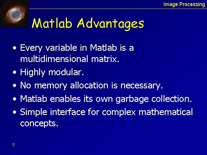
Image Processing Matlab Advantages • Every variable in Matlab is a multidimensional matrix. • Highly modular. • No memory allocation is necessary. • Matlab enables its own garbage collection. • Simple interface for complex mathematical concepts. 5

Image Processing Getting Help >> help (explain how to get help) >> helpbrowser / doc (open the online Matlab documentation) >> help images (list of all commands in the Image Processing Toolbox) >> demo >> lookfor read (display list of function with ‘read’ in the name or help text) >> type imread >> help imread (function name + % block) >> doc imread (function documentation in help browser) • Using [tab] is useful to auto-complete function names and variables • Mathworks website: http: //www. mathworks. com/products/matlab 6

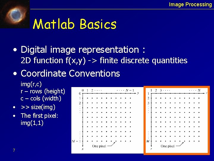
Image Processing Matlab Basics • Digital image representation : 2 D function f(x, y) -> finite discrete quantities • Coordinate Conventions img(r, c) r – rows (height) c – cols (width) • >> size(img) • The first pixel: img(1, 1) 7

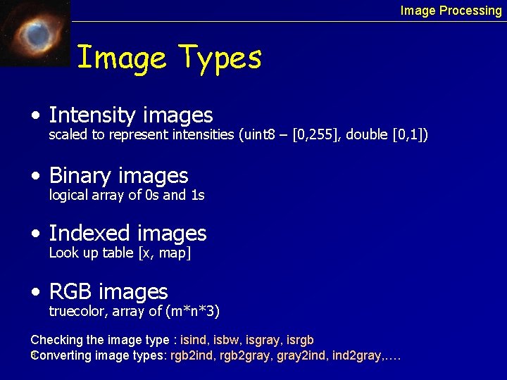
Image Processing Image Types • Intensity images scaled to represent intensities (uint 8 – [0, 255], double [0, 1]) • Binary images logical array of 0 s and 1 s • Indexed images Look up table [x, map] • RGB images truecolor, array of (m*n*3) Checking the image type : isind, isbw, isgray, isrgb 8 Converting image types: rgb 2 ind, rgb 2 gray, gray 2 ind, ind 2 gray, ….

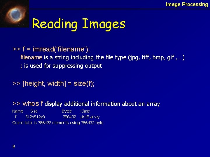
Image Processing Reading Images >> f = imread(‘filename’); filename is a string including the file type (jpg, tiff, bmp, gif , …) ; is used for suppressing output >> [height, width] = size(f); >> whos f display additional information about an array Name Size Bytes Class f 512 x 3 786432 uint 8 array Grand total is 786432 elements using 786432 byte 9

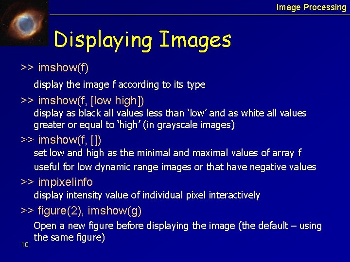
Image Processing Displaying Images >> imshow(f) display the image f according to its type >> imshow(f, [low high]) display as black all values less than ‘low’ and as white all values greater or equal to ‘high’ (in grayscale images) >> imshow(f, []) set low and high as the minimal and maximal values of array f useful for low dynamic range images or that have negative values >> impixelinfo display intensity value of individual pixel interactively >> figure(2), imshow(g) 10 Open a new figure before displaying the image (the default – using the same figure)

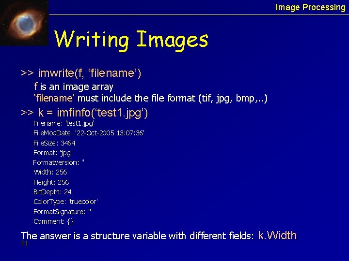
Image Processing Writing Images >> imwrite(f, ‘filename’) f is an image array ‘filename’ must include the file format (tif, jpg, bmp, . . ) >> k = imfinfo(‘test 1. jpg’) Filename: 'test 1. jpg' File. Mod. Date: '22 -Oct-2005 13: 07: 36' File. Size: 3464 Format: 'jpg' Format. Version: '' Width: 256 Height: 256 Bit. Depth: 24 Color. Type: 'truecolor' Format. Signature: '' Comment: {} The answer is a structure variable with different fields: 11 k. Width

Image Processing Data Classes 12 Converting between types : B = data_class_name(A) for example: B = double(A)

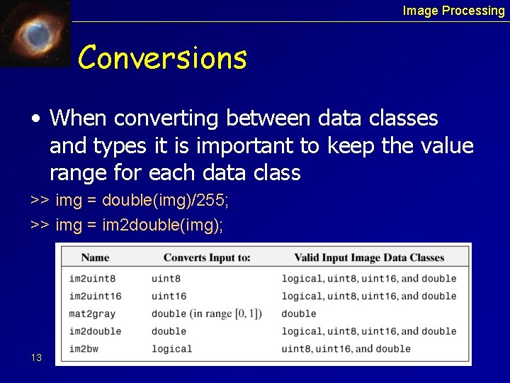
Image Processing Conversions • When converting between data classes and types it is important to keep the value range for each data class >> img = double(img)/255; >> img = im 2 double(img); 13

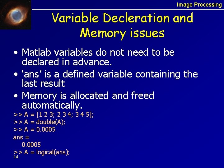
Image Processing Variable Decleration and Memory issues • Matlab variables do not need to be declared in advance. • ‘ans’ is a defined variable containing the last result • Memory is allocated and freed automatically. >> A = [1 2 3; 2 3 4; 3 4 5]; >> A = double(A); >> A = 0. 0005 ans = 0. 0005 >> A = logical(ans); 14

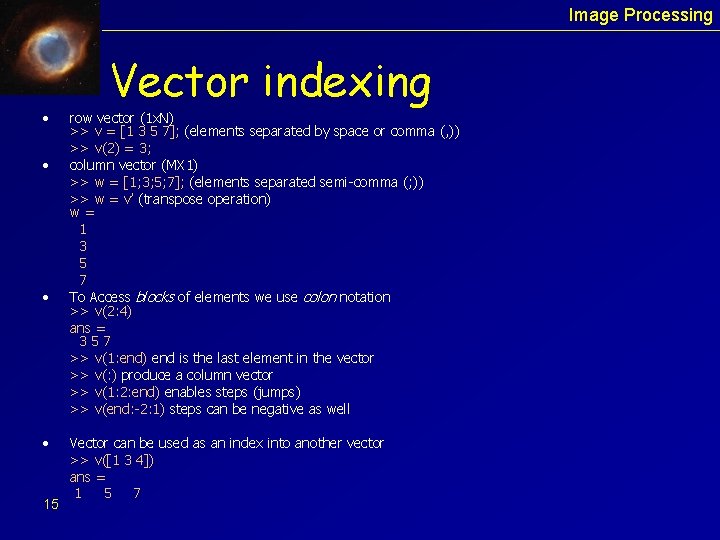
Image Processing • • 15 Vector indexing row vector (1 x. N) >> v = [1 3 5 7]; (elements separated by space or comma (, )) >> v(2) = 3; column vector (MX 1) >> w = [1; 3; 5; 7]; (elements separated semi-comma (; )) >> w = v’ (transpose operation) w= 1 3 5 7 To Access blocks of elements we use colon notation >> v(2: 4) ans = 357 >> v(1: end) end is the last element in the vector >> v(: ) produce a column vector >> v(1: 2: end) enables steps (jumps) >> v(end: -2: 1) steps can be negative as well Vector can be used as an index into another vector >> v([1 3 4]) ans = 1 5 7

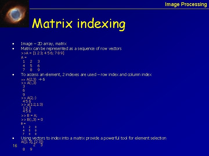
Image Processing Matrix indexing • • • Image – 2 D array, matrix Matrix can be represented as a sequence of row vectors >>A A= 1 4 7 = [1 2 3; 4 5 6; 7 8 9] 2 5 8 3 6 9 To access an element, 2 indexes are used – row index and column index A(2, 3) 6 >> A(: , 3) 3 6 9 >> A(2, : ) 456 >> a(1: 2, 1: 3) 123 456 >> B = A; >> B(: , 3) = 0 >> • 16 B= 1 4 7 2 5 8 0 0 0 Using vectors to index into a matrix provide a powerful tool for element selection A([1 3], [2 3]) 2 3 8 9

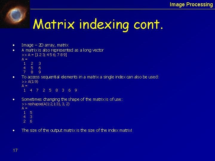
Image Processing Matrix indexing cont. • • Image – 2 D array, matrix A matrix is also represented as a long vector • To access sequential elements in a matrix a single index can also be used: >> A = [1 2 3; 4 5 6; 7 8 9] A= 1 2 3 4 5 6 7 8 9 >> A(1: 9) A= 1 4 7 2 5 8 3 6 9 • Sometimes changing the shape of the matrix is of use: • The size of the output matrix is the size of the index matrix! 17 >> reshapse(A(1: 2, 1: 3), 3, 2) A= 1 5 4 3 2 6

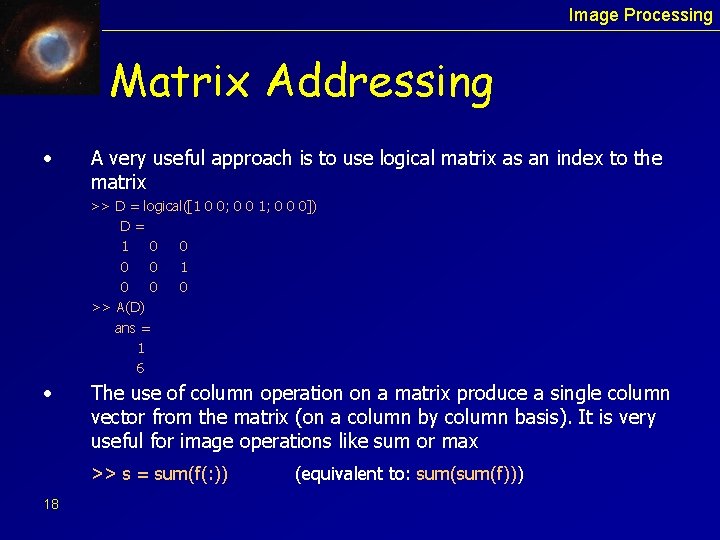
Image Processing Matrix Addressing • A very useful approach is to use logical matrix as an index to the matrix >> D = logical([1 0 0; 0 0 1; 0 0 0]) D= 1 0 0 0 >> A(D) ans = 1 6 • The use of column operation on a matrix produce a single column vector from the matrix (on a column by column basis). It is very useful for image operations like sum or max >> s = sum(f(: )) 18 (equivalent to: sum(f)))

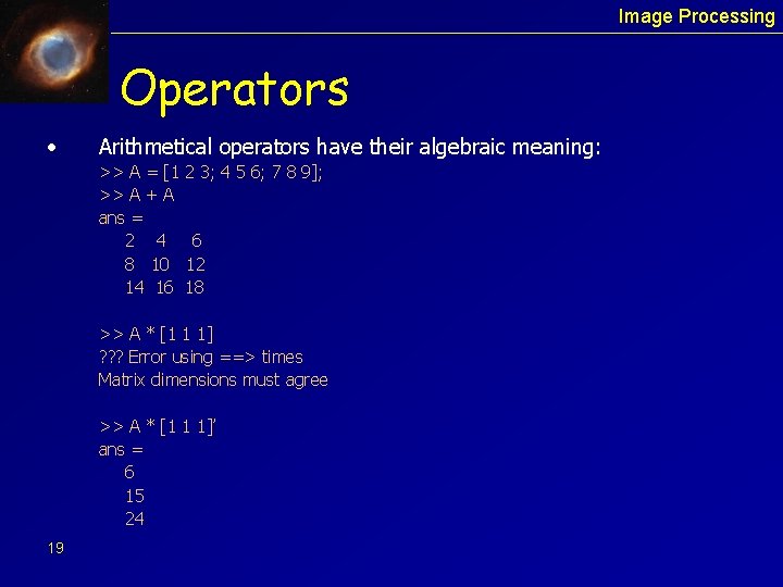
Image Processing Operators • Arithmetical operators have their algebraic meaning: >> A = [1 2 3; 4 5 6; 7 8 9]; >> A + A ans = 2 4 6 8 10 12 14 16 18 >> A * [1 1 1] ? ? ? Error using ==> times Matrix dimensions must agree >> A * [1 1 1]’ ans = 6 15 24 19

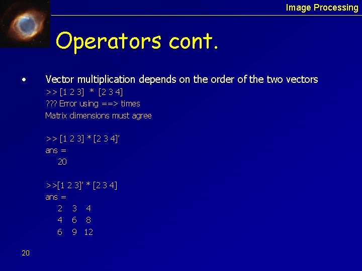
Image Processing Operators cont. • Vector multiplication depends on the order of the two vectors >> [1 2 3] * [2 3 4] ? ? ? Error using ==> times Matrix dimensions must agree >> [1 2 3] * [2 3 4]’ ans = 20 >>[1 2 3]’ * [2 3 4] ans = 2 3 4 4 6 8 6 9 12 20

Image Processing Operators cont. • Element by element operators >> [1 2 3]. * [2 3 4] ans = 2 6 12 >> [1 2 3]. ^ 2 ans = 1 4 9 >> [1 2 3]. / (2: 2: 6) ans = 0. 5000 21 . *. ^. /

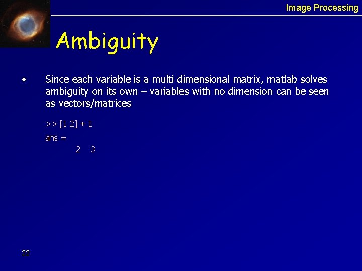
Image Processing Ambiguity • Since each variable is a multi dimensional matrix, matlab solves ambiguity on its own – variables with no dimension can be seen as vectors/matrices >> [1 2] + 1 ans = 2 22 3

Image Processing Array dimensions • Matlab arrays can be of any dimensions • It is useful to operate on specific dimension of the array, for example: >> height = size(i, 1); • Usually we deal with 2 D arrays but there are cases we need to address higher dimensions (such as color images) >> i(200: 300, 200: 400, 3) • To get the number of dimensions of an array >> d = ndims(f) 23

Image Processing Standard Arrays • Generating simple array enables trying out simple ideas and test the syntax of a function during development >> zeros(m, n) >> ones(m, n) >> true(m, n) >> false(m, n) >> magic(m) >> rand(n) >> randn(n) >> pascal(n) 24

Image Processing Additional Operators • Arithmetic operators (numeric computations) – matrix arithmetic (linear algebra A*B) – array arithmetic (element by element A. *B) +, -, . /, . ^, : . . • Relational operators (compare) – Compare corresponding elements of arrays of equal dimensions (<, >, <=, >=, ==, ~=) or an array to scalar • Logical operators can operate both on logical and numeric data (and: &, or: |, not: ~) true: logical 1 or non-zero numeric quantity false: logical or numerical 0 25 logical functions : xor, any, all

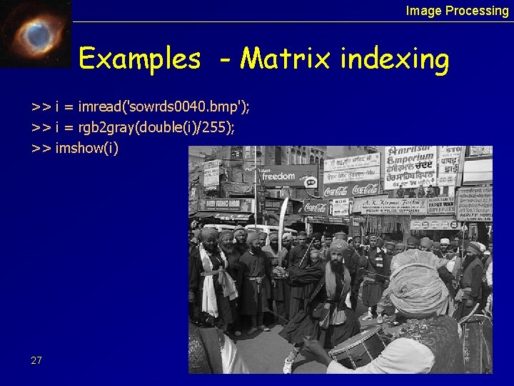
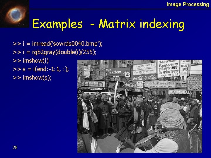
Image Processing Examples - Matrix indexing >> i = imread('sowrds 0040. bmp'); >> i = rgb 2 gray(double(i)/255); >> imshow(i) 26

Image Processing Examples - Matrix indexing >> i = imread('sowrds 0040. bmp'); >> i = rgb 2 gray(double(i)/255); >> imshow(i) 27

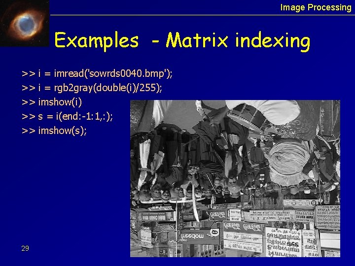
Image Processing Examples - Matrix indexing >> >> >> 28 i = imread('sowrds 0040. bmp'); i = rgb 2 gray(double(i)/255); imshow(i) s = i(end: -1: 1, : ); imshow(s);

Image Processing Examples - Matrix indexing >> >> >> 29 i = imread('sowrds 0040. bmp'); i = rgb 2 gray(double(i)/255); imshow(i) s = i(end: -1: 1, : ); imshow(s);

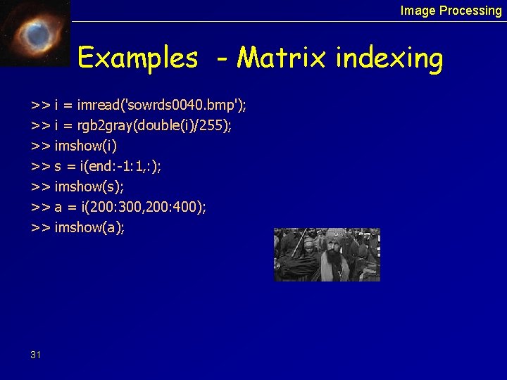
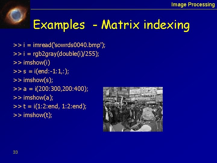
Image Processing Examples - Matrix indexing >> >> 30 i = imread('sowrds 0040. bmp'); i = rgb 2 gray(double(i)/255); imshow(i) s = i(end: -1: 1, : ); imshow(s); a = i(200: 300, 200: 400); imshow(a);

Image Processing Examples - Matrix indexing >> >> 31 i = imread('sowrds 0040. bmp'); i = rgb 2 gray(double(i)/255); imshow(i) s = i(end: -1: 1, : ); imshow(s); a = i(200: 300, 200: 400); imshow(a);

Image Processing Examples - Matrix indexing >> >> >> 32 i = imread('sowrds 0040. bmp'); i = rgb 2 gray(double(i)/255); imshow(i) s = i(end: -1: 1, : ); imshow(s); a = i(200: 300, 200: 400); imshow(a); t = i(1: 2: end, 1: 2: end); imshow(t);

Image Processing Examples - Matrix indexing >> >> >> 33 i = imread('sowrds 0040. bmp'); i = rgb 2 gray(double(i)/255); imshow(i) s = i(end: -1: 1, : ); imshow(s); a = i(200: 300, 200: 400); imshow(a); t = i(1: 2: end, 1: 2: end); imshow(t);

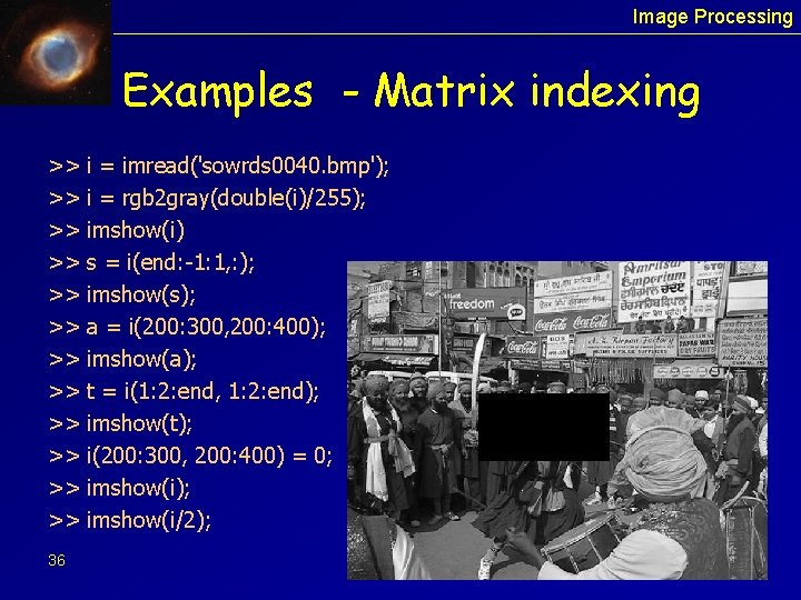
Image Processing Examples - Matrix indexing >> >> >> 34 i = imread('sowrds 0040. bmp'); i = rgb 2 gray(double(i)/255); imshow(i) s = i(end: -1: 1, : ); imshow(s); a = i(200: 300, 200: 400); imshow(a); t = i(1: 2: end, 1: 2: end); imshow(t); i(200: 300, 200: 400) = 0; imshow(i);

Image Processing Examples - Matrix indexing >> >> >> 35 i = imread('sowrds 0040. bmp'); i = rgb 2 gray(double(i)/255); imshow(i) s = i(end: -1: 1, : ); imshow(s); a = i(200: 300, 200: 400); imshow(a); t = i(1: 2: end, 1: 2: end); imshow(t); i(200: 300, 200: 400) = 0; imshow(i);

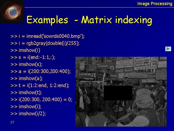
Image Processing Examples - Matrix indexing >> >> >> 36 i = imread('sowrds 0040. bmp'); i = rgb 2 gray(double(i)/255); imshow(i) s = i(end: -1: 1, : ); imshow(s); a = i(200: 300, 200: 400); imshow(a); t = i(1: 2: end, 1: 2: end); imshow(t); i(200: 300, 200: 400) = 0; imshow(i); imshow(i/2);

Image Processing Examples - Matrix indexing >> >> >> 37 i = imread('sowrds 0040. bmp'); i = rgb 2 gray(double(i)/255); imshow(i) s = i(end: -1: 1, : ); imshow(s); a = i(200: 300, 200: 400); imshow(a); t = i(1: 2: end, 1: 2: end); imshow(t); i(200: 300, 200: 400) = 0; imshow(i); imshow(i/2);

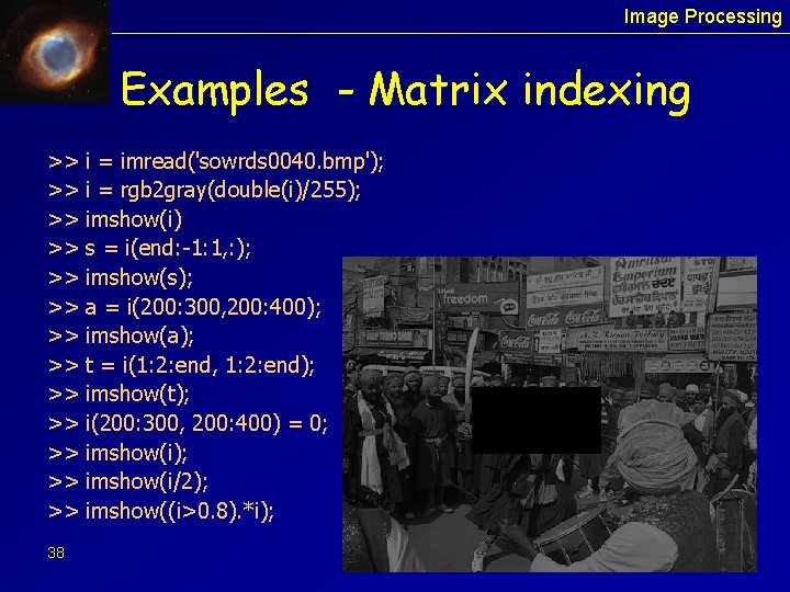
Image Processing Examples - Matrix indexing >> >> >> >> 38 i = imread('sowrds 0040. bmp'); i = rgb 2 gray(double(i)/255); imshow(i) s = i(end: -1: 1, : ); imshow(s); a = i(200: 300, 200: 400); imshow(a); t = i(1: 2: end, 1: 2: end); imshow(t); i(200: 300, 200: 400) = 0; imshow(i); imshow(i/2); imshow((i>0. 8). *i);

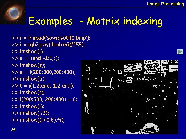
Image Processing Examples - Matrix indexing >> >> >> >> 39 i = imread('sowrds 0040. bmp'); i = rgb 2 gray(double(i)/255); imshow(i) s = i(end: -1: 1, : ); imshow(s); a = i(200: 300, 200: 400); imshow(a); t = i(1: 2: end, 1: 2: end); imshow(t); i(200: 300, 200: 400) = 0; imshow(i); imshow(i/2); imshow((i>0. 8). *i);

Image Processing M-Files can be one of two: • Scripts – A series of commands that are performed on the global scope. No input and output variables. • Functions – A set of commands performed over a given input, with a required output. Functions have a scope of their own. (accessing the global scope can be done by defining the variables to be ‘globals’). In both types – the m-file must be in the current directory, or in a previously added path (added with the function addpath) 40

Image Processing M-Function Programming Components of m files: • Function definition line function [out 1 out 2] = name(in 1, in 2, in 3) • H 1 line - a single comment line that follows the function definition line. % SQUARESUM compute the sum of the square of the matrix elements This line appears when user writes >> help function_name >> lookfor keyword - display all functions where the keyword appeared in H 1 line 41

Image Processing M-Function Programming • Components of m files (cont. ): • Help Text - text block following the H 1 line without any blank line in between the two • Function body – the Matlab code • Comments – lines starting with % Note: – add short and clear comments to your code! 42

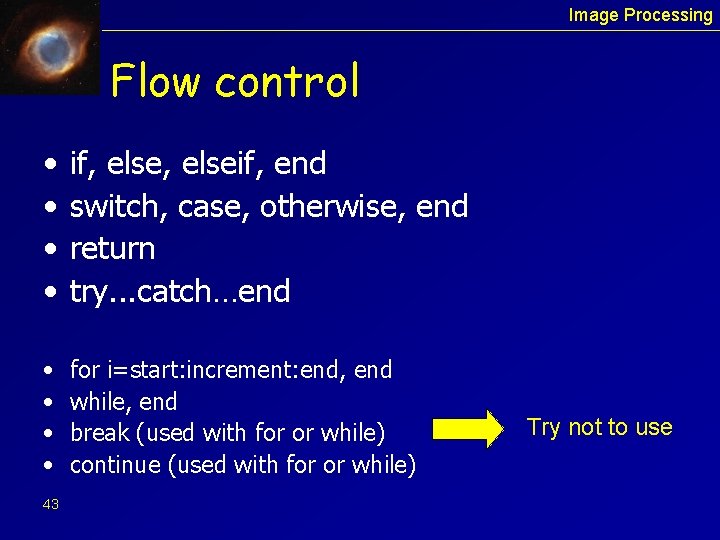
Image Processing Flow control • • if, elseif, end switch, case, otherwise, end return try. . . catch…end • • for i=start: increment: end, end while, end break (used with for or while) continue (used with for or while) 43 Try not to use

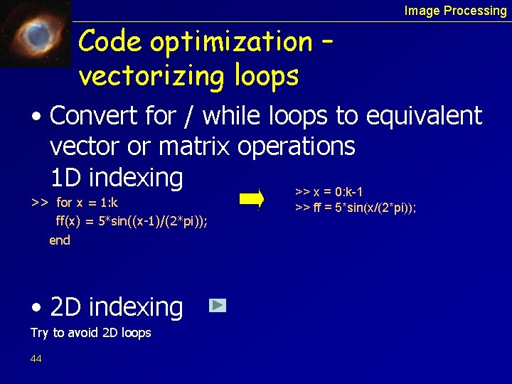
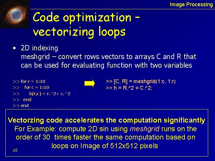
Image Processing Code optimization – vectorizing loops • Convert for / while loops to equivalent vector or matrix operations 1 D indexing >> x = 0: k-1 >> for x = 1: k ff(x) = 5*sin((x-1)/(2*pi)); end • 2 D indexing Try to avoid 2 D loops 44 >> ff = 5*sin(x/(2*pi));

Image Processing Code optimization – vectorizing loops • 2 D indexing meshgrid – convert rows vectors to arrays C and R that can be used for evaluating function with two variables >> for r = 1: 10 >> for c = 1: 10 >> b(r, c) = r. ^2+ c. ^2 >> end >> [C, R] = meshgrid(1: c, 1: r) >> h = R. ^2 + C. ^2; Vectorzing code accelerates the computation significantly For Example: compute 2 D sin using meshgrid runs on the order of 30 times faster the same computation based on loops on Image of 512 x 512 pixels 45

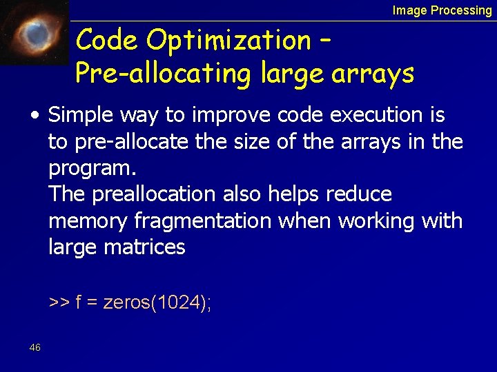
Image Processing Code Optimization – Pre-allocating large arrays • Simple way to improve code execution is to pre-allocate the size of the arrays in the program. The preallocation also helps reduce memory fragmentation when working with large matrices >> f = zeros(1024); 46

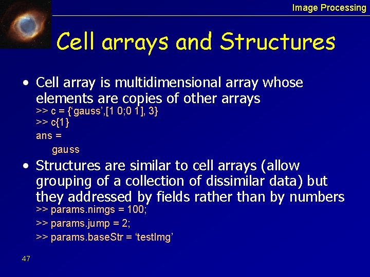
Image Processing Cell arrays and Structures • Cell array is multidimensional array whose elements are copies of other arrays >> c = {‘gauss’, [1 0; 0 1], 3} >> c{1} ans = gauss • Structures are similar to cell arrays (allow grouping of a collection of dissimilar data) but they addressed by fields rather than by numbers >> params. nimgs = 100; >> params. jump = 2; >> params. base. Str = ‘test. Img’ 47

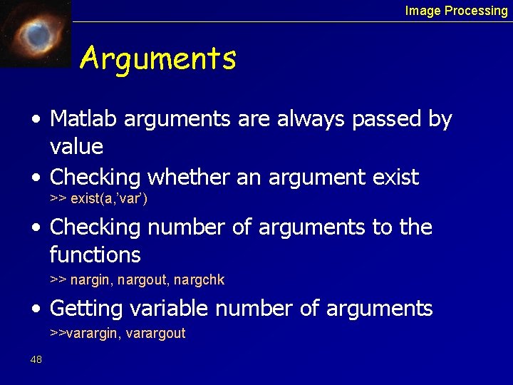
Image Processing Arguments • Matlab arguments are always passed by value • Checking whether an argument exist >> exist(a, ’var’) • Checking number of arguments to the functions >> nargin, nargout, nargchk • Getting variable number of arguments >>varargin, varargout 48

Image Processing Gui >> guide (Graphic User Interface Development Environment) Start the GUI Layout Editor. Guide create – fig file: complete description of the gui elements and their arrangements – gui m-file: the code that controls the gui operations, initializations functions, callback functions 49

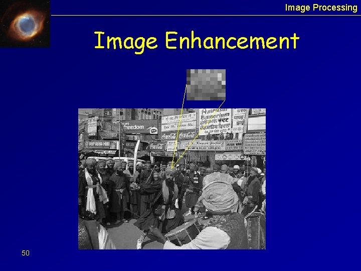
Image Processing Image Enhancement 50

Image Processing Intensity Transformation • Spatial Domain – image plane itself direct manipulation of pixels in the image. g(x, y) = T(f(x, y)) • T is an operator of f, defined over a specific neighborhood around a pixel. • Principle approach – use a square around the pixel. In the simplest case the square size is one pixel 51

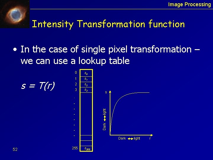
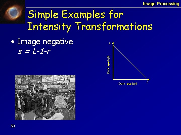
Image Processing Intensity Transformation function • In the case of single pixel transformation – we can use a lookup table s = T(r) 0 s 0 1 s 1 2 s 2 3 s 3 . 52 255 Dark light . . . . s Dark s 255 light r

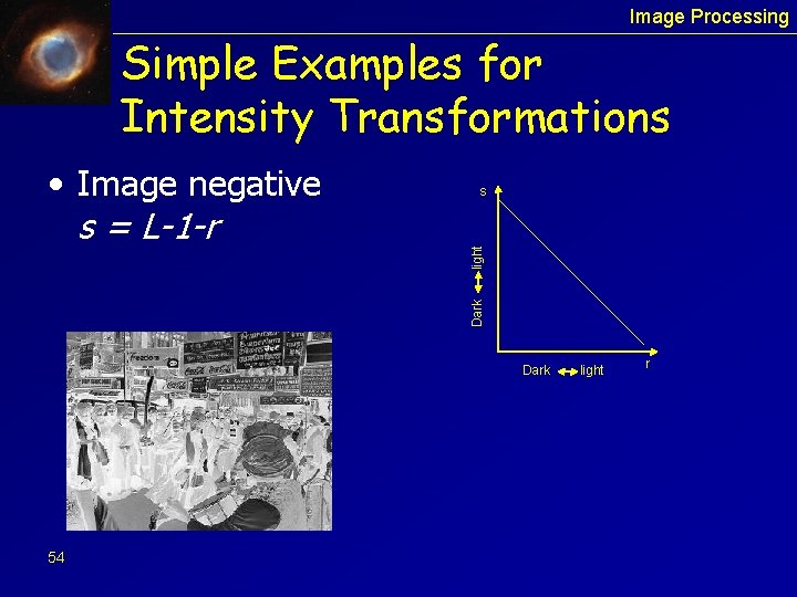
Image Processing Simple Examples for Intensity Transformations light s Dark • Image negative s = L-1 -r Dark 53 light r

Image Processing Simple Examples for Intensity Transformations light s Dark • Image negative s = L-1 -r Dark 54 light r

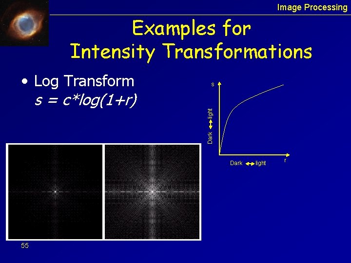
Image Processing Examples for Intensity Transformations light s Dark • Log Transform s = c*log(1+r) Dark 55 light r

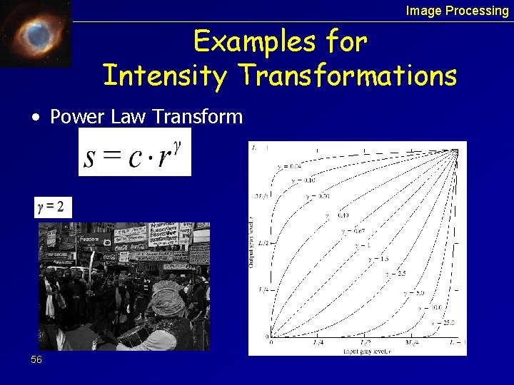
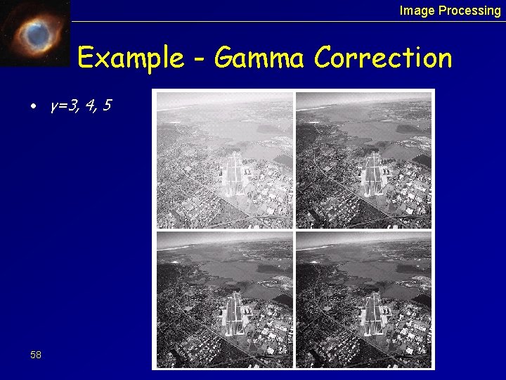
Image Processing Examples for Intensity Transformations • Power Law Transform 56

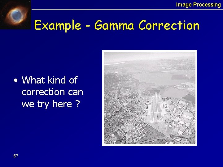
Image Processing Example - Gamma Correction • What kind of correction can we try here ? 57

Image Processing Example - Gamma Correction • γ=3, 4, 5 58

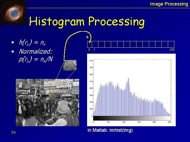
Image Processing Histogram Processing • h(rk) = nk • Normalized: p(rk) = nk/N 59 + 0 1 in Matlab: imhist(img) 255

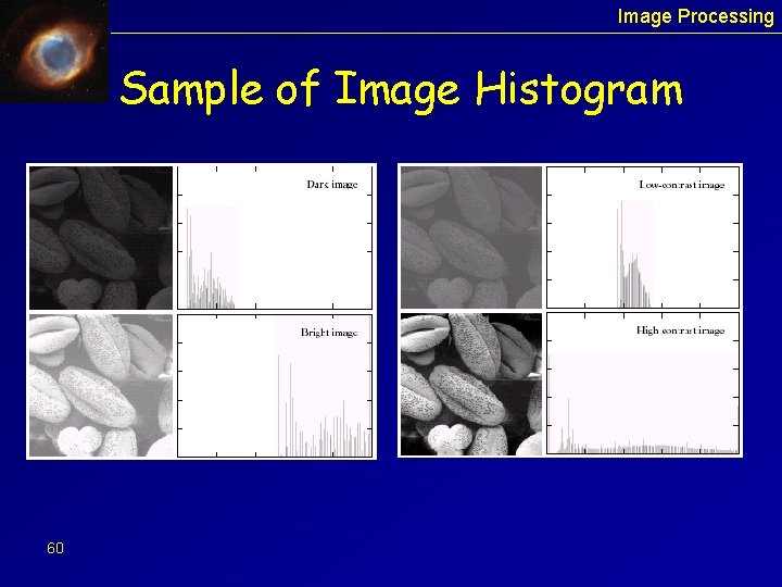
Image Processing Sample of Image Histogram 60

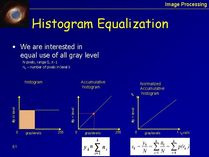
Image Processing Histogram Equalization • We are interested in equal use of all gray level N pixels, range 0, . . K-1 nk – number of pixels in level k histogram Accumulative histogram 0 61 graylevels 255 1 #p < level #p in level sk Normalized Accumulative histogram 0 graylevels 255 0 graylevels 1 rk=k/K

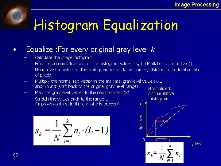
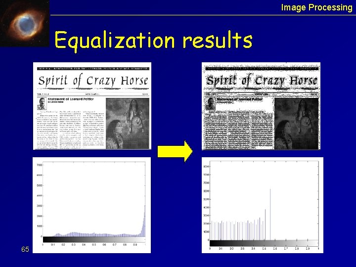
Image Processing Histogram Equalization • Equalize : For every original gray level k – – #p < level – – Calculate the image histogram Find the accumulative sum of the histogram values - yk (in Matlab – cumsum(vec)) Normalize the values of the histogram accumulative sum by dividing in the total number of pixels Multiply the normalized vector in the maximal gray level value (K-1) and round (shift back to the original gray level range) Normalized Map the gray level values to the result of step (3) Accumulative histogram Stretch the values back to the range 1, . . K 1 s k (improve contrast in the end of this process) 0 62 rk sk 1 rk=k/K

Image Processing Histogram Equalization • In most discrete images it is impossible to obtain uniform histogram, we want to get as close as possible to uniform. • The distribution of gray levels in areas along the histogram will result in approximately same number of pixels • The number of bins can only decrease: bins can never split and small bins in the histogram may be united (but the effect is not visibly disturbing since it involves a very small number of pixels) • The histogram equalization process is monotonic (as the process involves accumulative sum) and therefore the relative brightness of a pixel is preserved 63

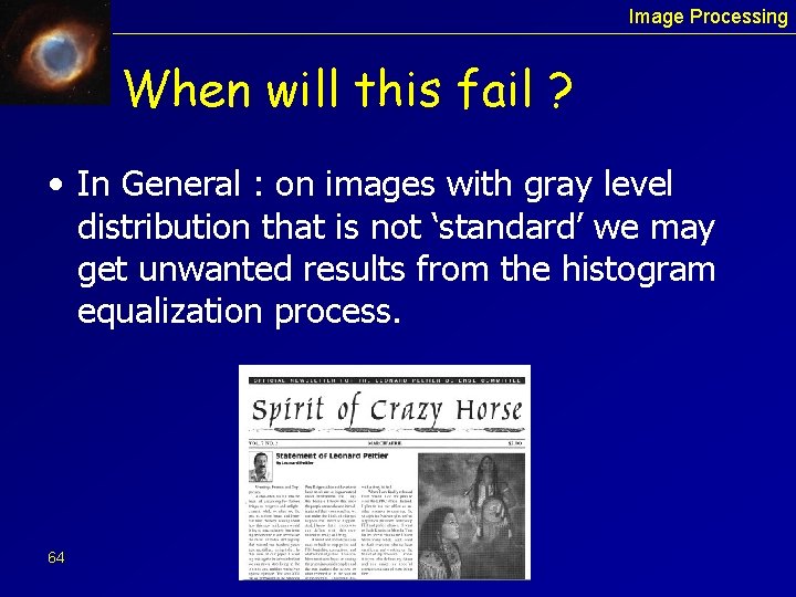
Image Processing When will this fail ? • In General : on images with gray level distribution that is not ‘standard’ we may get unwanted results from the histogram equalization process. 64

Image Processing Equalization results 65

Image Processing Exercise 1 • Targets: – Getting familiar with the Matlab environment – Learning image formats and conversions between them – Argument error checking – Working with image histograms – Writing an efficient code 66

Image Processing A few more important commands for image operations (look in the help) • • 67 find repmat reshape clear save plot, subplot disp