Digital Image Processing Image Enhancement Point Processing 2

Digital Image Processing Image Enhancement (Point Processing)

2 of 45 Contents In this lecture we will look at image enhancement point processing techniques: – What is point processing? – Negative images – Thresholding – Logarithmic transformation – Power law transforms – Grey level slicing – Bit plane slicing

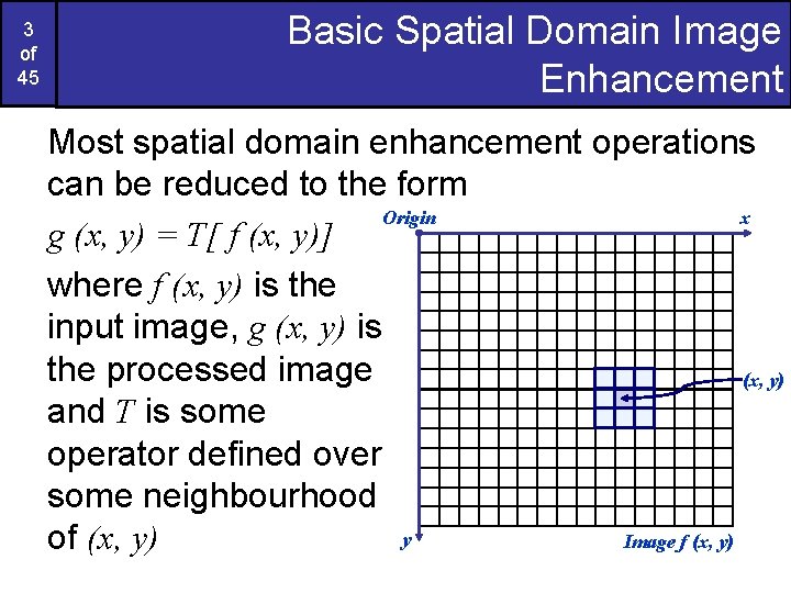
3 of 45 Basic Spatial Domain Image Enhancement Most spatial domain enhancement operations can be reduced to the form Origin x g (x, y) = T[ f (x, y)] where f (x, y) is the input image, g (x, y) is the processed image (x, y) and T is some operator defined over some neighbourhood y Image f (x, y) of (x, y)

4 of 45 Point Processing The simplest spatial domain operations occur when the neighbourhood is simply the pixel itself In this case T is referred to as a grey level transformation function or a point processing operation Point processing operations take the form s=T(r) where s refers to the processed image pixel value and r refers to the original image pixel value

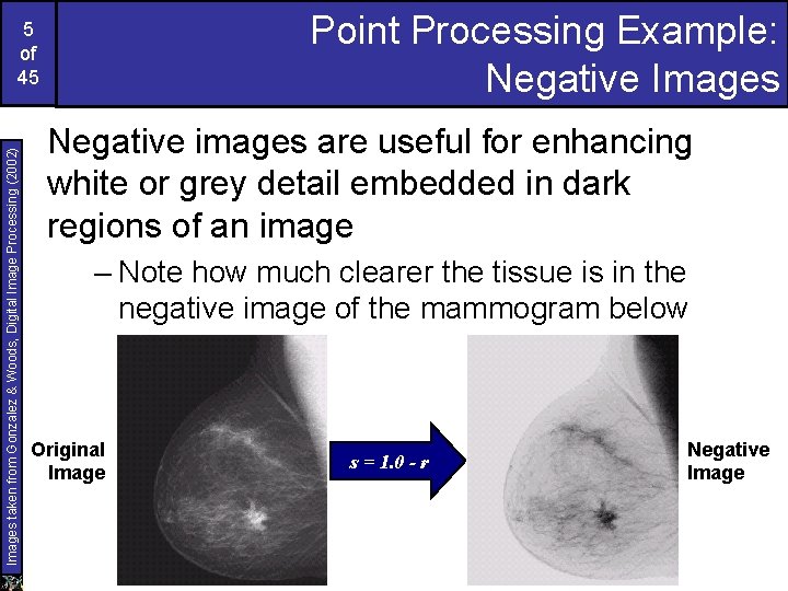
Point Processing Example: Negative Images taken from Gonzalez & Woods, Digital Image Processing (2002) 5 of 45 Negative images are useful for enhancing white or grey detail embedded in dark regions of an image – Note how much clearer the tissue is in the negative image of the mammogram below Original Image s = 1. 0 - r Negative Image

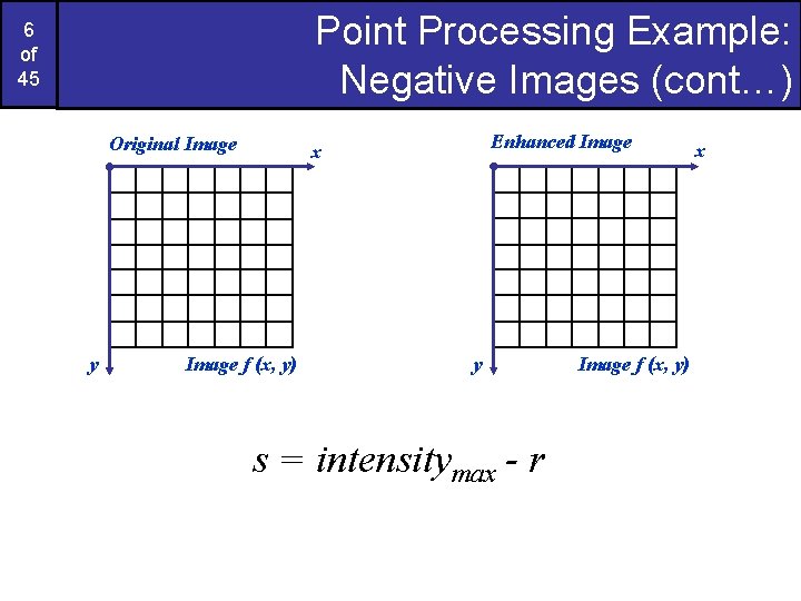
Point Processing Example: Negative Images (cont…) 6 of 45 Original Image y Enhanced Image x Image f (x, y) y s = intensitymax - r Image f (x, y) x

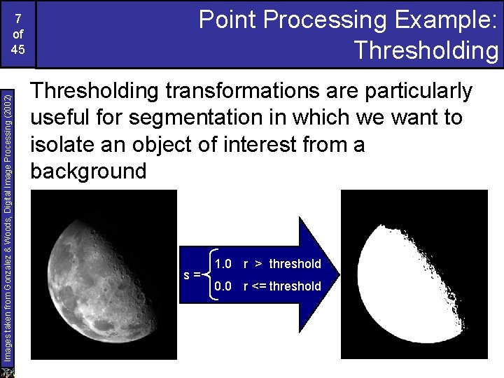
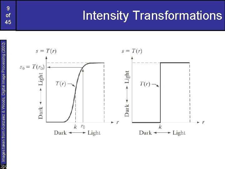
Images taken from Gonzalez & Woods, Digital Image Processing (2002) 7 of 45 Point Processing Example: Thresholding transformations are particularly useful for segmentation in which we want to isolate an object of interest from a background s = 1. 0 r > threshold 0. 0 r <= threshold

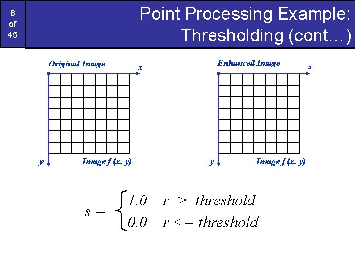
Point Processing Example: Thresholding (cont…) 8 of 45 Original Image y Image f (x, y) s= Enhanced Image x 1. 0 0. 0 y Image f (x, y) r > threshold r <= threshold x

Images taken from Gonzalez & Woods, Digital Image Processing (2002) 9 of 45 Intensity Transformations

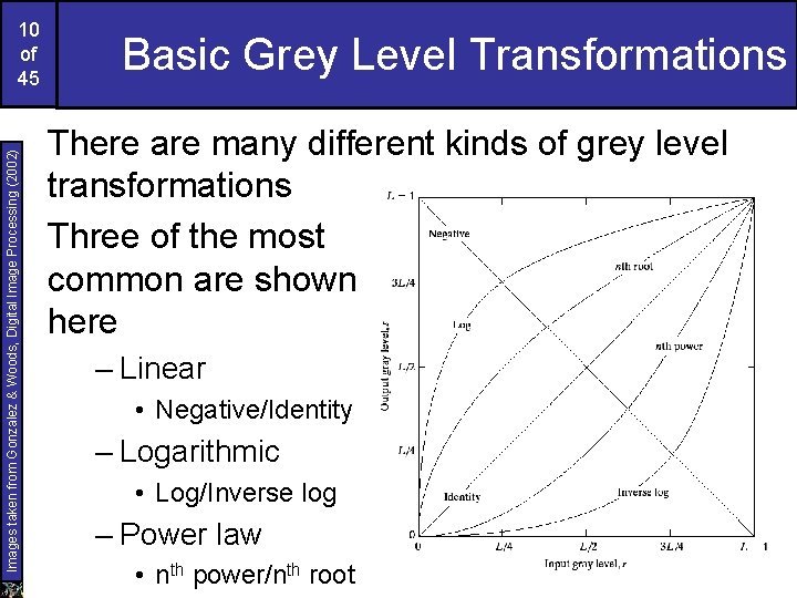
Images taken from Gonzalez & Woods, Digital Image Processing (2002) 10 of 45 Basic Grey Level Transformations There are many different kinds of grey level transformations Three of the most common are shown here – Linear • Negative/Identity – Logarithmic • Log/Inverse log – Power law • nth power/nth root

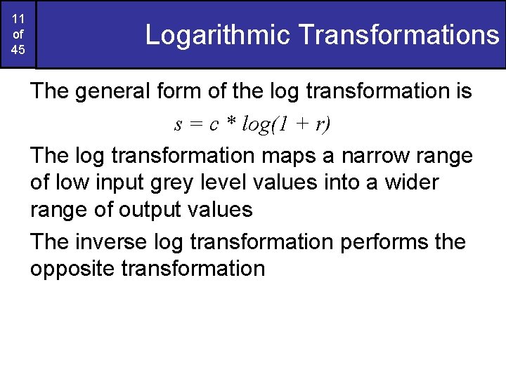
11 of 45 Logarithmic Transformations The general form of the log transformation is s = c * log(1 + r) The log transformation maps a narrow range of low input grey level values into a wider range of output values The inverse log transformation performs the opposite transformation

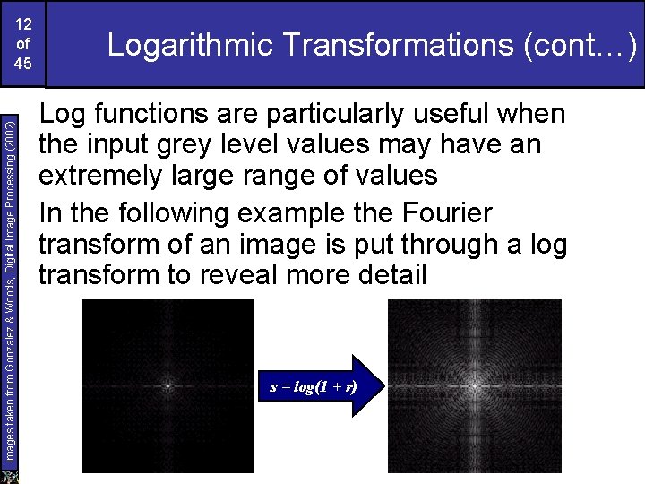
Images taken from Gonzalez & Woods, Digital Image Processing (2002) 12 of 45 Logarithmic Transformations (cont…) Log functions are particularly useful when the input grey level values may have an extremely large range of values In the following example the Fourier transform of an image is put through a log transform to reveal more detail s = log(1 + r)

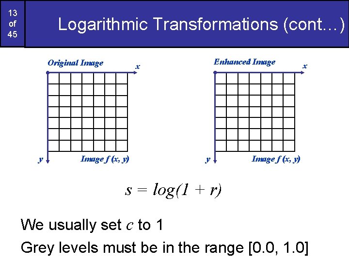
13 of 45 Logarithmic Transformations (cont…) Original Image y Enhanced Image x Image f (x, y) y x Image f (x, y) s = log(1 + r) We usually set c to 1 Grey levels must be in the range [0. 0, 1. 0]

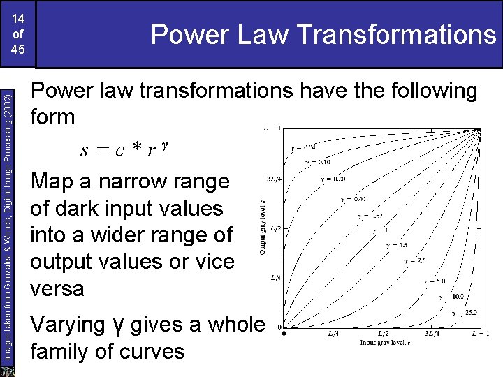
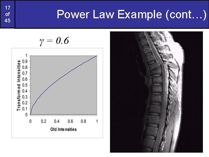
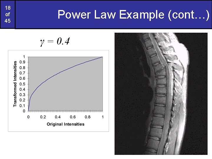
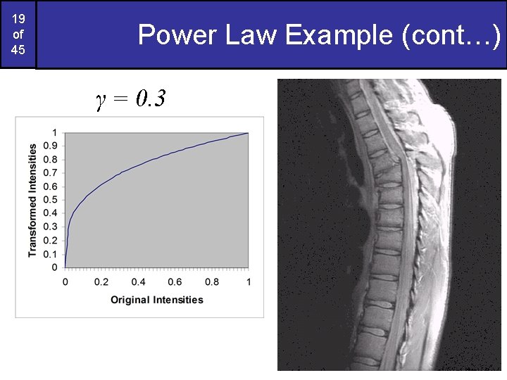
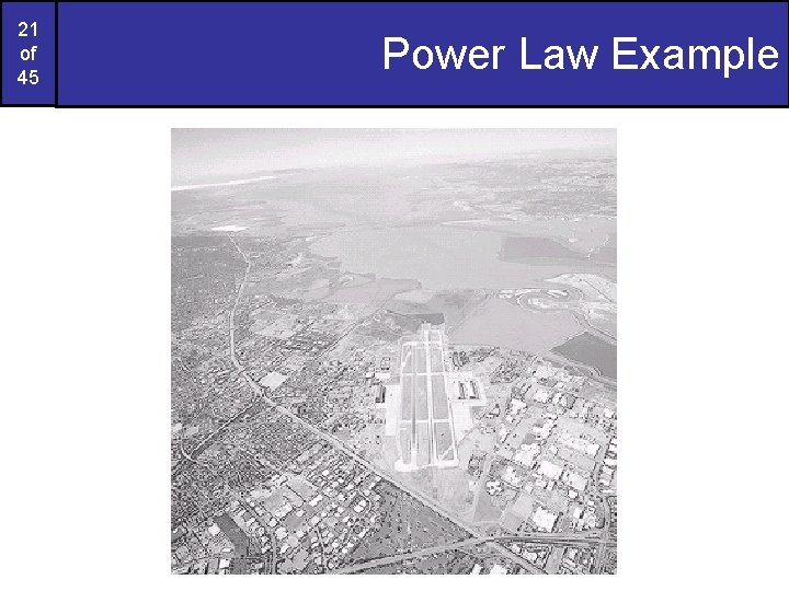
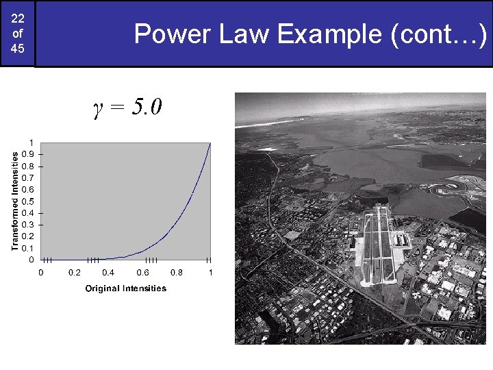
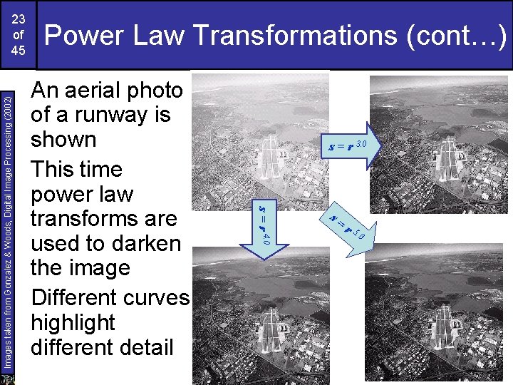
Images taken from Gonzalez & Woods, Digital Image Processing (2002) 14 of 45 Power Law Transformations Power law transformations have the following form s=c*rγ Map a narrow range of dark input values into a wider range of output values or vice versa Varying γ gives a whole family of curves

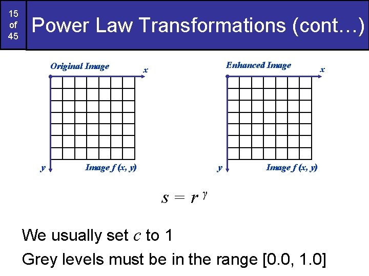
15 of 45 Power Law Transformations (cont…) Original Image y Enhanced Image x y Image f (x, y) x Image f (x, y) s=rγ We usually set c to 1 Grey levels must be in the range [0. 0, 1. 0]

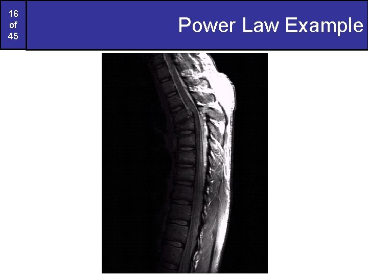
16 of 45 Power Law Example

17 of 45 Power Law Example (cont…) γ = 0. 6

18 of 45 Power Law Example (cont…) γ = 0. 4

19 of 45 Power Law Example (cont…) γ = 0. 3

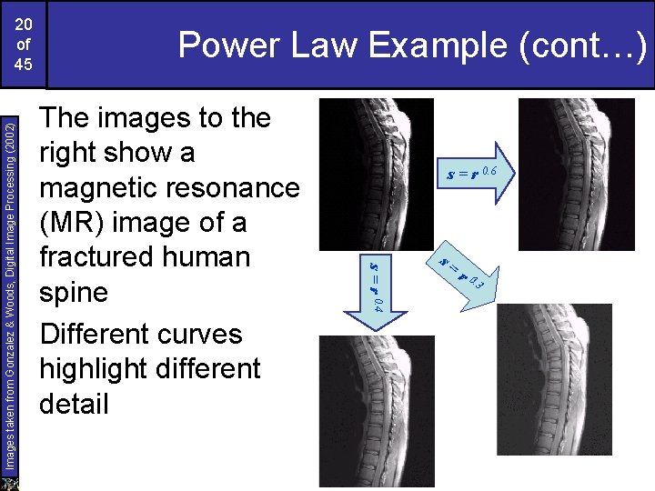
Power Law Example (cont…) The images to the right show a magnetic resonance (MR) image of a fractured human spine Different curves highlight different detail s = r 0. 6 s = r 0. 4 Images taken from Gonzalez & Woods, Digital Image Processing (2002) 20 of 45 s= r 0. 3

21 of 45 Power Law Example

22 of 45 Power Law Example (cont…) γ = 5. 0

Power Law Transformations (cont…) An aerial photo of a runway is shown This time power law transforms are used to darken the image Different curves highlight different detail s = r 3. 0 s = r 4. 0 Images taken from Gonzalez & Woods, Digital Image Processing (2002) 23 of 45 s= r 5. 0

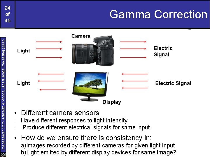
Images taken from Gonzalez & Woods, Digital Image Processing (2002) 24 of 45 Gamma Correction • Different camera sensors - Have different responses to light intensity - Produce different electrical signals for same input • How do we ensure there is consistency in: a)Images recorded by different cameras for given light input b)Light emitted by different display devices for same image?

Images taken from Gonzalez & Woods, Digital Image Processing (2002) 25 of 45 Gamma Correction • What is the relation between: Camera: Light on sensor vs. “intensity” of corre sponding pixel Display: Pixel intensity vs. light from that pixel • Relation between pixel value and corre sponding physical quantity is usually complex, nonlinear

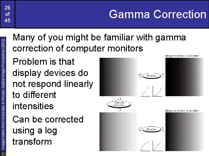
Images taken from Gonzalez & Woods, Digital Image Processing (2002) 26 of 45 Gamma Correction Many of you might be familiar with gamma correction of computer monitors Problem is that display devices do not respond linearly to different intensities Can be corrected using a log transform

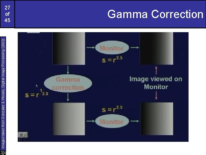
Images taken from Gonzalez & Woods, Digital Image Processing (2002) 27 of 45 Gamma Correction

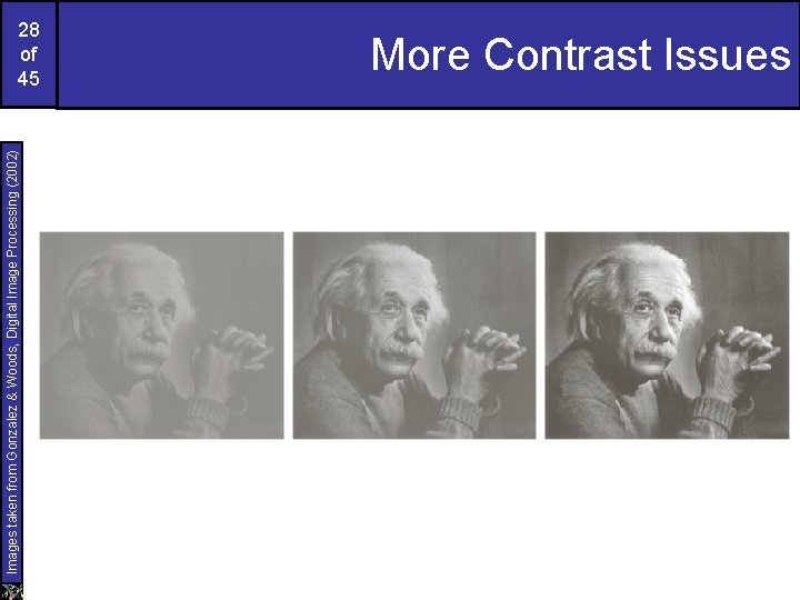
Images taken from Gonzalez & Woods, Digital Image Processing (2002) 28 of 45 More Contrast Issues

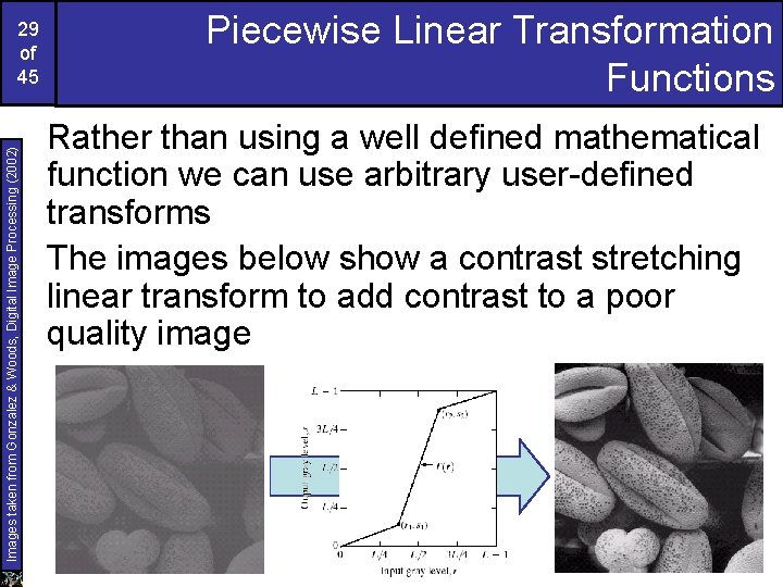
Images taken from Gonzalez & Woods, Digital Image Processing (2002) 29 of 45 Piecewise Linear Transformation Functions Rather than using a well defined mathematical function we can use arbitrary user-defined transforms The images below show a contrast stretching linear transform to add contrast to a poor quality image

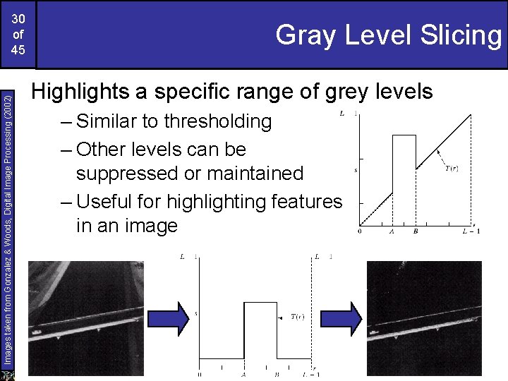
Images taken from Gonzalez & Woods, Digital Image Processing (2002) 30 of 45 Gray Level Slicing Highlights a specific range of grey levels – Similar to thresholding – Other levels can be suppressed or maintained – Useful for highlighting features in an image

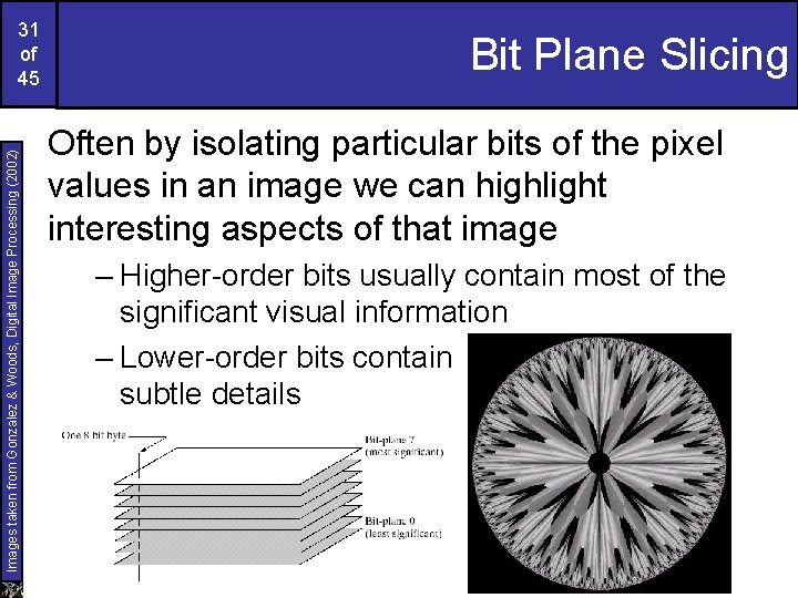
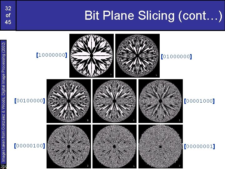
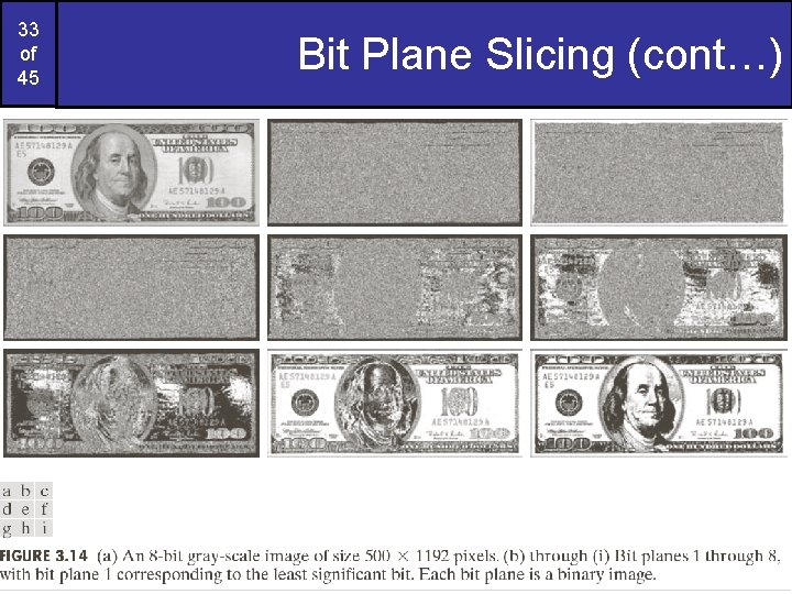
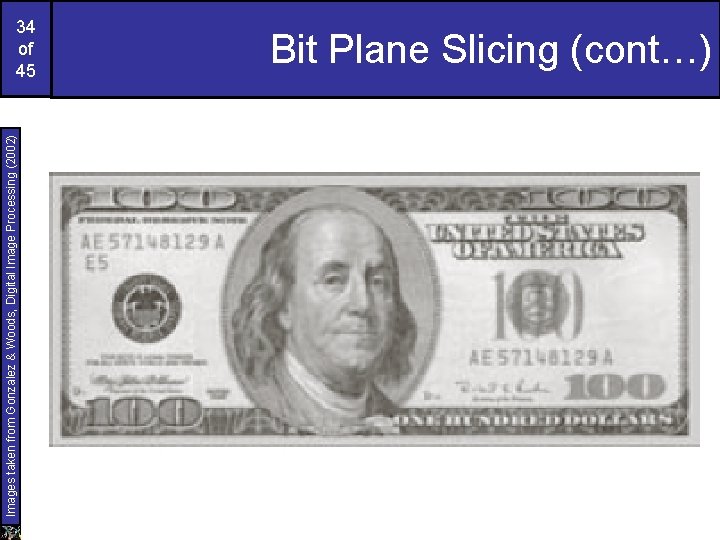
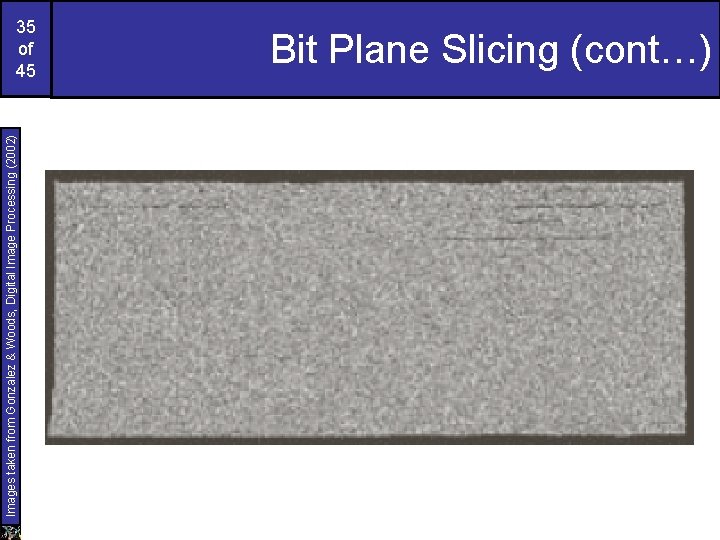
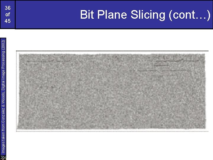
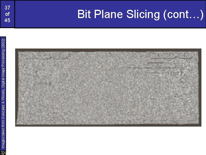
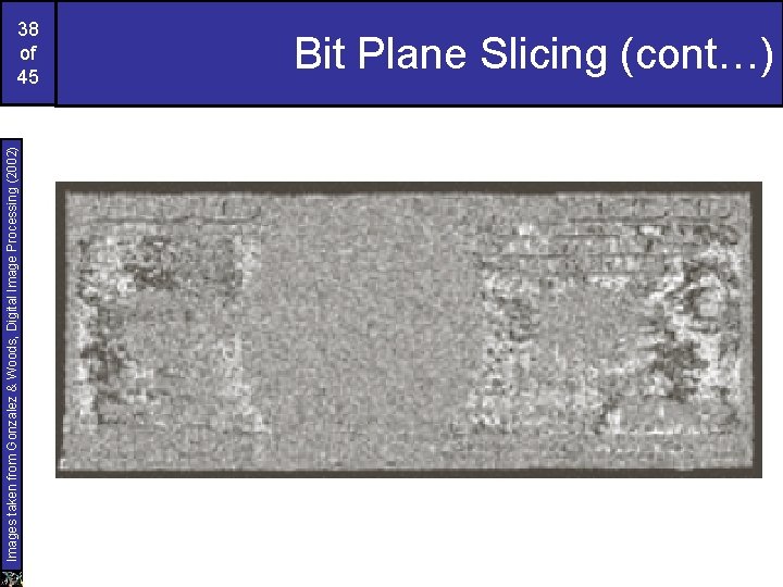
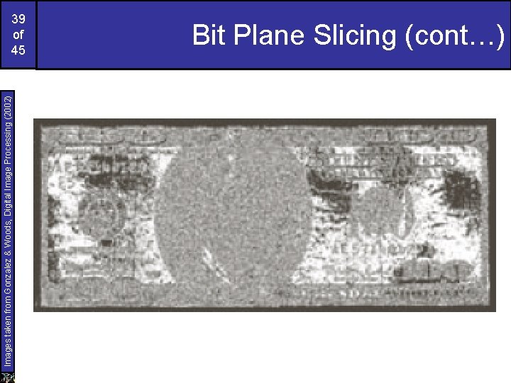
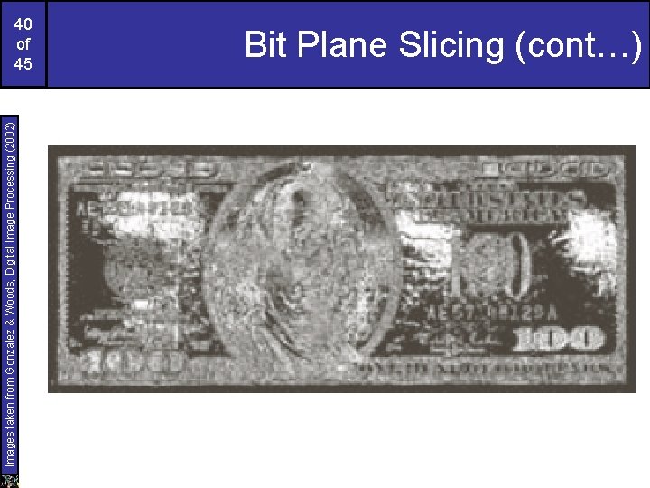
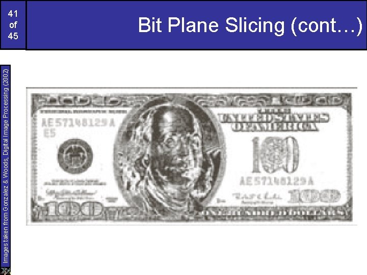
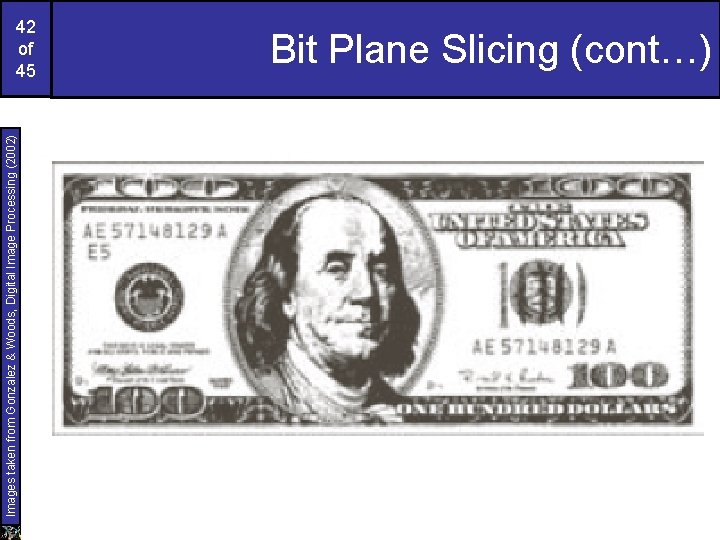
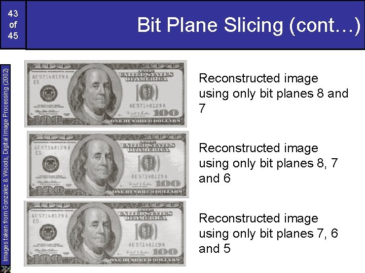
Images taken from Gonzalez & Woods, Digital Image Processing (2002) 31 of 45 Bit Plane Slicing Often by isolating particular bits of the pixel values in an image we can highlight interesting aspects of that image – Higher-order bits usually contain most of the significant visual information – Lower-order bits contain subtle details

Images taken from Gonzalez & Woods, Digital Image Processing (2002) 32 of 45 Bit Plane Slicing (cont…) [10000000] [01000000] [00100000] [00001000] [00000100] [00000001]

33 of 45 Bit Plane Slicing (cont…)

Images taken from Gonzalez & Woods, Digital Image Processing (2002) 34 of 45 Bit Plane Slicing (cont…)

Images taken from Gonzalez & Woods, Digital Image Processing (2002) 35 of 45 Bit Plane Slicing (cont…)

Images taken from Gonzalez & Woods, Digital Image Processing (2002) 36 of 45 Bit Plane Slicing (cont…)

Images taken from Gonzalez & Woods, Digital Image Processing (2002) 37 of 45 Bit Plane Slicing (cont…)

Images taken from Gonzalez & Woods, Digital Image Processing (2002) 38 of 45 Bit Plane Slicing (cont…)

Images taken from Gonzalez & Woods, Digital Image Processing (2002) 39 of 45 Bit Plane Slicing (cont…)

Images taken from Gonzalez & Woods, Digital Image Processing (2002) 40 of 45 Bit Plane Slicing (cont…)

Images taken from Gonzalez & Woods, Digital Image Processing (2002) 41 of 45 Bit Plane Slicing (cont…)

Images taken from Gonzalez & Woods, Digital Image Processing (2002) 42 of 45 Bit Plane Slicing (cont…)

Images taken from Gonzalez & Woods, Digital Image Processing (2002) 43 of 45 Bit Plane Slicing (cont…) Reconstructed image using only bit planes 8 and 7 Reconstructed image using only bit planes 8, 7 and 6 Reconstructed image using only bit planes 7, 6 and 5

44 of 45 Report Histogram Specification

45 of 45 Summary We have looked at different kinds of point processing image enhancement Next time we will start to look at neighbourhood operations – in particular filtering and convolution