Image Processing Ch 3 Intensity Transformation and spatial

Image Processing Ch 3: Intensity Transformation and spatial filters Part 2 Prepared by: Tahani Khatib

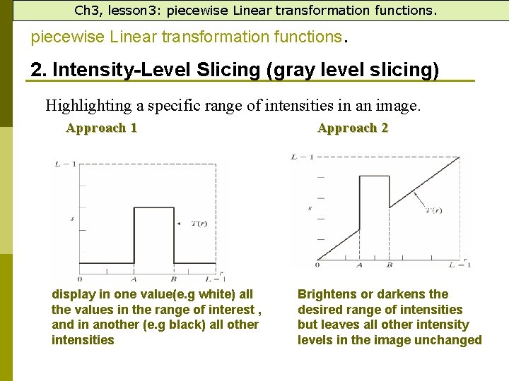
Ch 3, lesson 3: piecewise Linear transformation functions. 2. Intensity-Level Slicing (gray level slicing) Highlighting a specific range of intensities in an image. Approach 1 display in one value(e. g white) all the values in the range of interest , and in another (e. g black) all other intensities Approach 2 Brightens or darkens the desired range of intensities but leaves all other intensity levels in the image unchanged

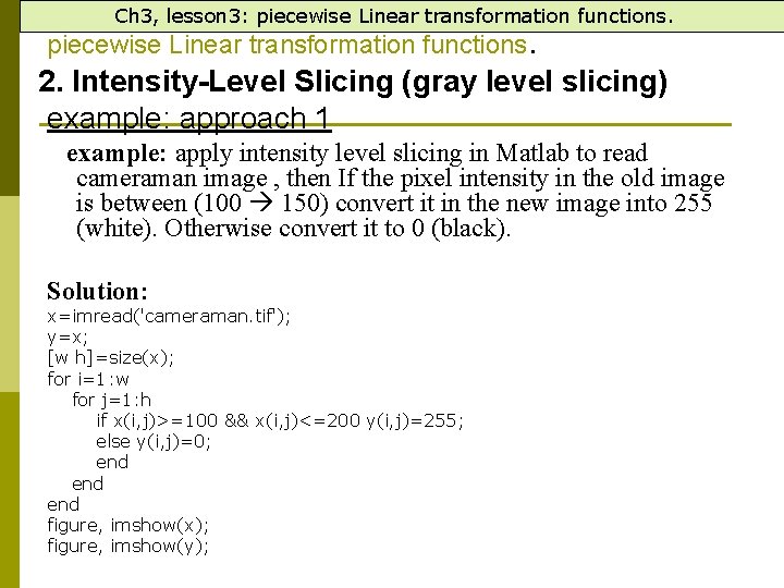
Ch 3, lesson 3: piecewise Linear transformation functions. 2. Intensity-Level Slicing (gray level slicing) example: approach 1 example: apply intensity level slicing in Matlab to read cameraman image , then If the pixel intensity in the old image is between (100 150) convert it in the new image into 255 (white). Otherwise convert it to 0 (black). Solution: x=imread('cameraman. tif'); y=x; [w h]=size(x); for i=1: w for j=1: h if x(i, j)>=100 && x(i, j)<=200 y(i, j)=255; else y(i, j)=0; end end figure, imshow(x); figure, imshow(y);

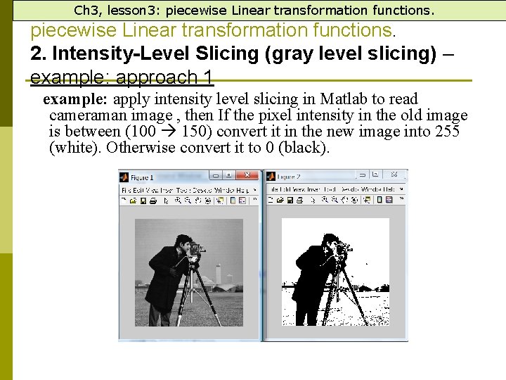
Ch 3, lesson 3: piecewise Linear transformation functions. 2. Intensity-Level Slicing (gray level slicing) – example: approach 1 example: apply intensity level slicing in Matlab to read cameraman image , then If the pixel intensity in the old image is between (100 150) convert it in the new image into 255 (white). Otherwise convert it to 0 (black).

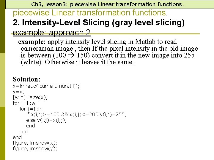
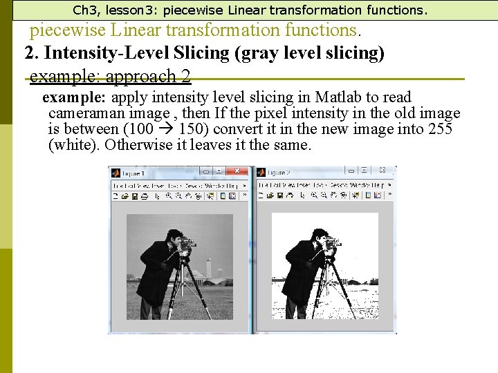
Ch 3, lesson 3: piecewise Linear transformation functions. 2. Intensity-Level Slicing (gray level slicing) example: approach 2 example: apply intensity level slicing in Matlab to read cameraman image , then If the pixel intensity in the old image is between (100 150) convert it in the new image into 255 (white). Otherwise it leaves it the same. Solution: x=imread('cameraman. tif'); y=x; [w h]=size(x); for i=1: w for j=1: h if x(i, j)>=100 && x(i, j)<=200 y(i, j)=255; else y(i, j)=x(i, j); end end figure, imshow(x); figure, imshow(y);

Ch 3, lesson 3: piecewise Linear transformation functions. 2. Intensity-Level Slicing (gray level slicing) example: approach 2 example: apply intensity level slicing in Matlab to read cameraman image , then If the pixel intensity in the old image is between (100 150) convert it in the new image into 255 (white). Otherwise it leaves it the same.

Ch 3, lesson 3: piecewise Linear transformation functions. 2. Intensity-Level Slicing (gray level slicing) Homework example: apply intensity level slicing (approch 2) in Matlab to read moon image , then If the pixel intensity in the old image is between (0 20) convert it in the new image into 130.

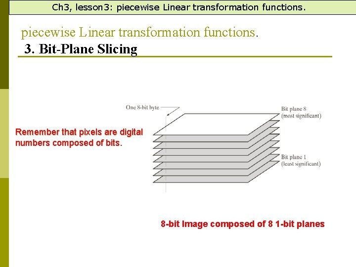
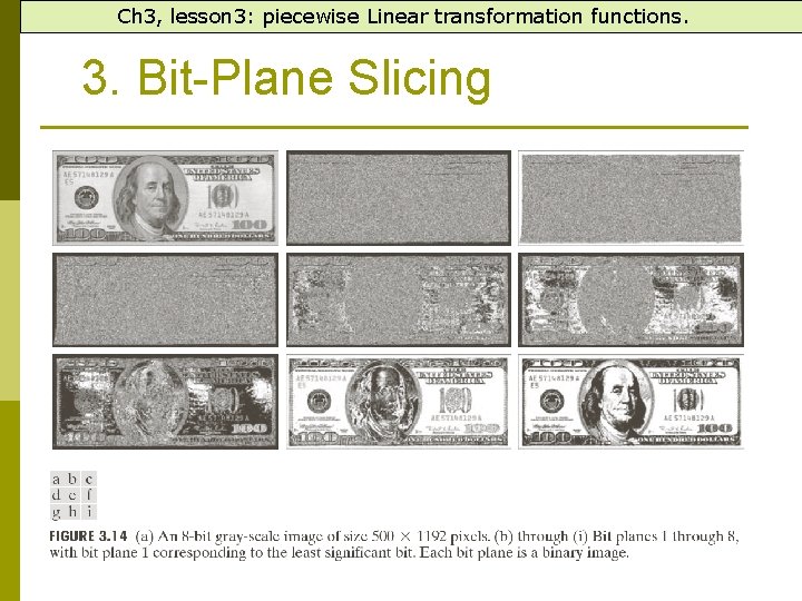
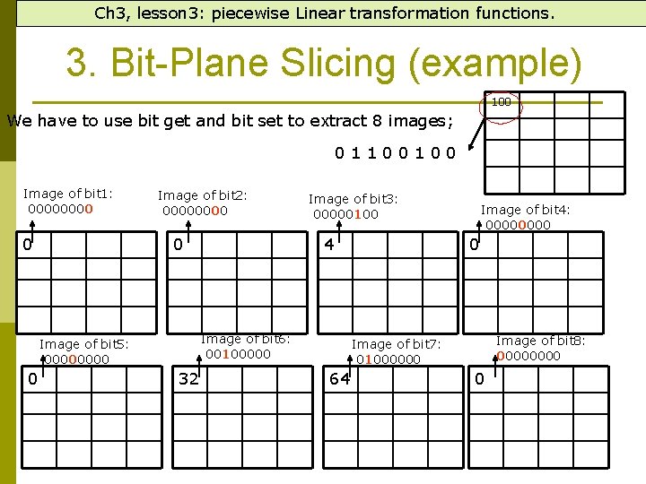
Ch 3, lesson 3: piecewise Linear transformation functions. 3. Bit-Plane Slicing Remember that pixels are digital numbers composed of bits. 8 -bit Image composed of 8 1 -bit planes

Ch 3, lesson 3: piecewise Linear transformation functions. 3. Bit-Plane Slicing

Ch 3, lesson 3: piecewise Linear transformation functions. 3. Bit-Plane Slicing (example) 100 We have to use bit get and bit set to extract 8 images; 01100100 Image of bit 1: 0000 0 Image of bit 2: 0000 0 4 Image of bit 6: 00100000 Image of bit 5: 0000 0 Image of bit 3: 00000100 32 Image of bit 4: 0000 0 Image of bit 8: 0000 Image of bit 7: 01000000 64 0

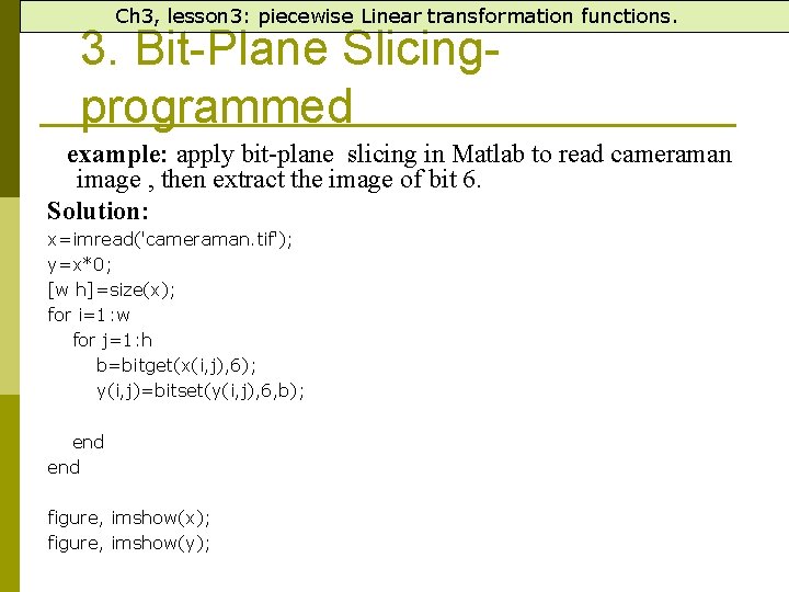
Ch 3, lesson 3: piecewise Linear transformation functions. 3. Bit-Plane Slicingprogrammed example: apply bit-plane slicing in Matlab to read cameraman image , then extract the image of bit 6. Solution: x=imread('cameraman. tif'); y=x*0; [w h]=size(x); for i=1: w for j=1: h b=bitget(x(i, j), 6); y(i, j)=bitset(y(i, j), 6, b); end figure, imshow(x); figure, imshow(y);

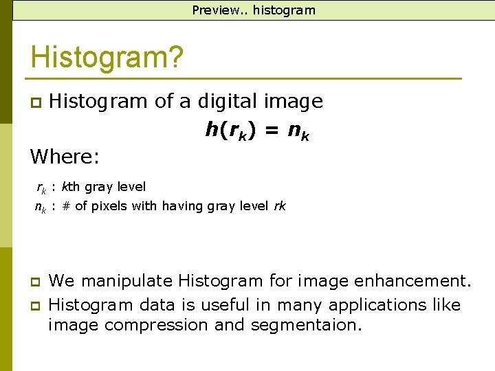
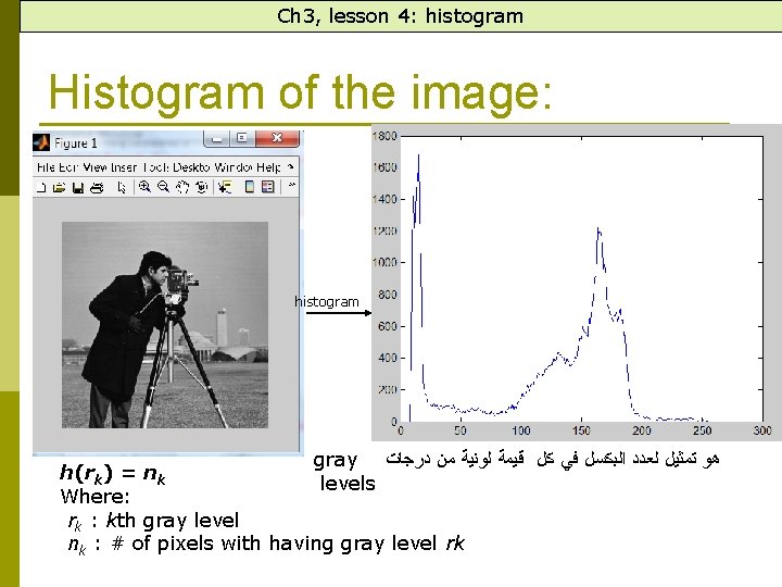
Preview. . histogram Histogram? Histogram of a digital image h(rk) = nk Where: p rk : kth gray level nk : # of pixels with having gray level rk p p We manipulate Histogram for image enhancement. Histogram data is useful in many applications like image compression and segmentaion.

Ch 3, lesson 4: histogram Histogram of the image: histogram gray ﻫﻮ ﺗﻤﺜﻴﻞ ﻟﻌﺪﺩ ﺍﻟﺒﻜﺴﻞ ﻓﻲ ﻛﻞ ﻗﻴﻤﺔ ﻟﻮﻧﻴﺔ ﻣﻦ ﺩﺭﺟﺎﺕ h ( rk ) = n k levels Where: rk : kth gray level nk : # of pixels with having gray level rk

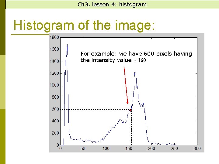
Ch 3, lesson 4: histogram Histogram of the image: For example: we have 600 pixels having the intensity value ≈ 160

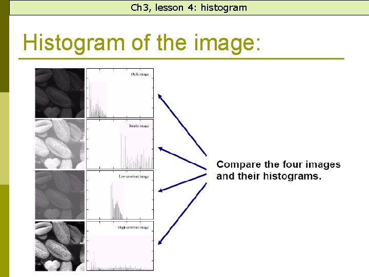
Ch 3, lesson 4: histogram Histogram of the image:

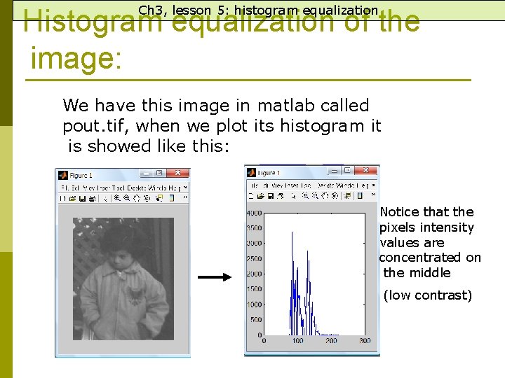
Ch 3, lesson 5: histogram equalization Histogram equalization of the image: We have this image in matlab called pout. tif, when we plot its histogram it is showed like this: Notice that the pixels intensity values are concentrated on the middle (low contrast)

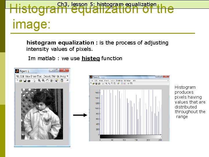
Ch 3, lesson 5: histogram equalization Histogram equalization of the image: histogram equalization : is the process of adjusting intensity values of pixels. Im matlab : we use histeq function Histogram produces pixels having values that are distributed throughout the range

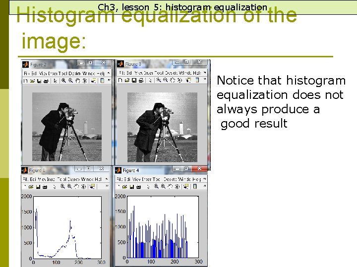
Ch 3, lesson 5: histogram equalization Histogram equalization of the image: Notice that histogram equalization does not always produce a good result

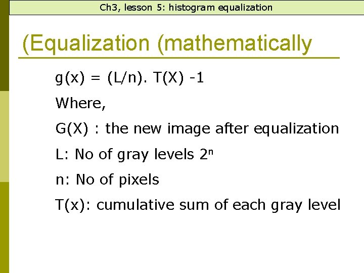
Ch 3, lesson 5: histogram equalization (Equalization (mathematically g(x) = (L/n). T(X) -1 Where, G(X) : the new image after equalization L: No of gray levels 2 n n: No of pixels T(x): cumulative sum of each gray level

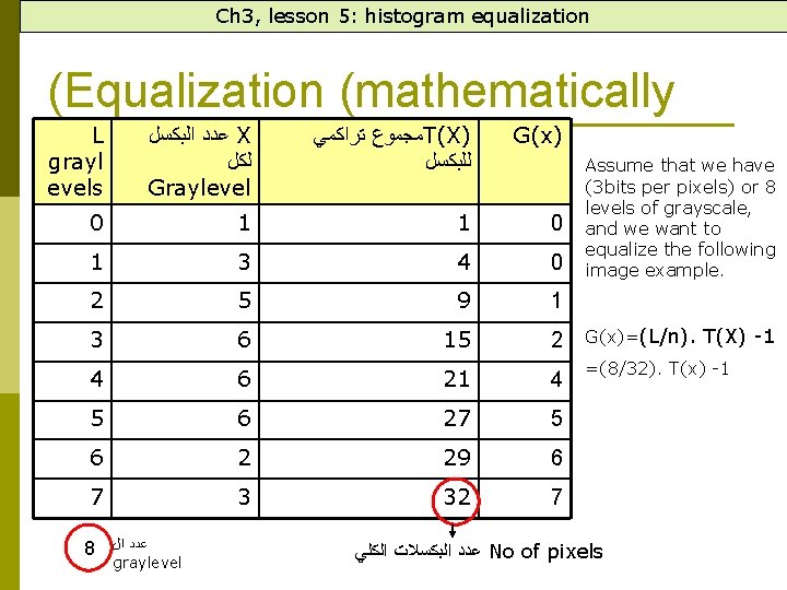
Ch 3, lesson 5: histogram equalization (Equalization (mathematically L grayl evels ﻋﺪﺩ ﺍﻟﺒﻜﺴﻞ X ﻟﻜﻞ Graylevel ﻣﺠﻤﻮﻉ ﺗﺮﺍﻛﻤﻲ T(X) ﻟﻠﺒﻜﺴﻞ G(x) 0 1 1 0 1 3 4 0 2 5 9 1 3 6 15 2 4 6 21 4 5 6 27 5 6 2 29 6 7 3 32 7 8 ﻋﺪﺩ ﺍﻝ graylevel Assume that we have (3 bits per pixels) or 8 levels of grayscale, and we want to equalize the following image example. G(x)=(L/n). T(X) -1 =(8/32). T(x) -1 ﻋﺪﺩ ﺍﻟﺒﻜﺴﻼﺕ ﺍﻟﻜﻠﻲ No of pixels