Digital Image Processing Lecture 4 Fundamentals Digital Image

Digital Image Processing Lecture 4: Fundamentals

Digital Image Representation • An image can be defined as a twodimensional function, f(x, y), where x and y are spatial (plane) coordinates, and the amplitude of f at any pair of coordinates (x, y) is called the intensity of the image at that point.

Digital Image Representation • An image may be continuous with respect to the xand y-coordinates, and also in amplitude (analogue). Converting such an image to digital form requires that the coordinates, as well as the amplitude, be digitized. Digitizing the coordinate values is called sampling; digitizing the amplitude values is called quantization. Thus, when x, y and f are all finite, discrete quantities, we call the image a digital image.

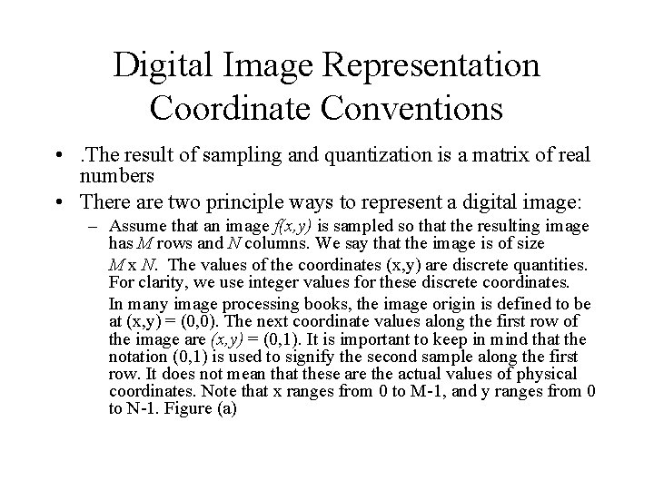
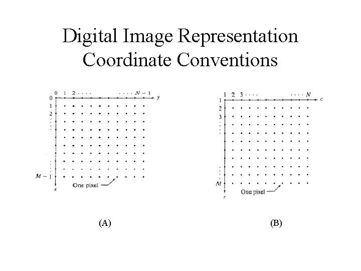
Digital Image Representation Coordinate Conventions • . The result of sampling and quantization is a matrix of real numbers • There are two principle ways to represent a digital image: – Assume that an image f(x, y) is sampled so that the resulting image has M rows and N columns. We say that the image is of size M x N. The values of the coordinates (x, y) are discrete quantities. For clarity, we use integer values for these discrete coordinates. In many image processing books, the image origin is defined to be at (x, y) = (0, 0). The next coordinate values along the first row of the image are (x, y) = (0, 1). It is important to keep in mind that the notation (0, 1) is used to signify the second sample along the first row. It does not mean that these are the actual values of physical coordinates. Note that x ranges from 0 to M-1, and y ranges from 0 to N-1. Figure (a)

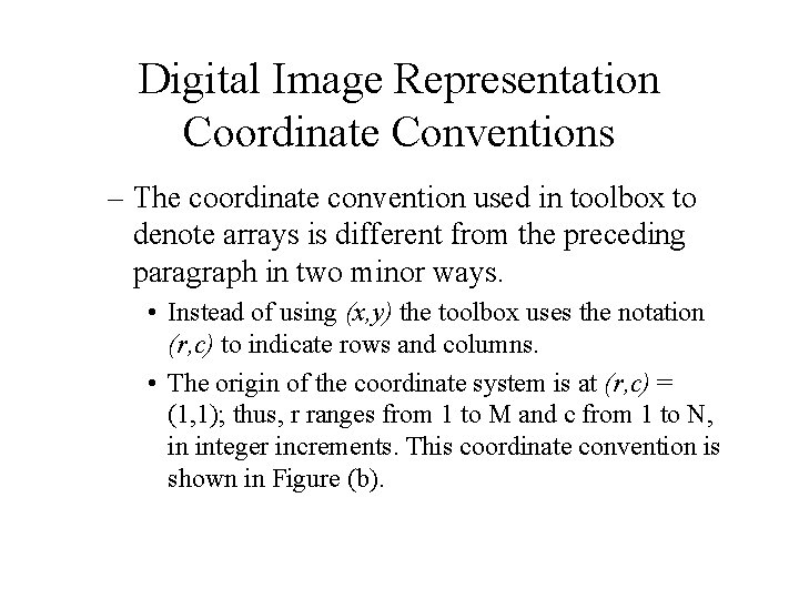
Digital Image Representation Coordinate Conventions – The coordinate convention used in toolbox to denote arrays is different from the preceding paragraph in two minor ways. • Instead of using (x, y) the toolbox uses the notation (r, c) to indicate rows and columns. • The origin of the coordinate system is at (r, c) = (1, 1); thus, r ranges from 1 to M and c from 1 to N, in integer increments. This coordinate convention is shown in Figure (b).

Digital Image Representation Coordinate Conventions (A) (B)

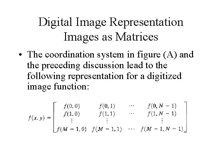
Digital Image Representation Images as Matrices • The coordination system in figure (A) and the preceding discussion lead to the following representation for a digitized image function:

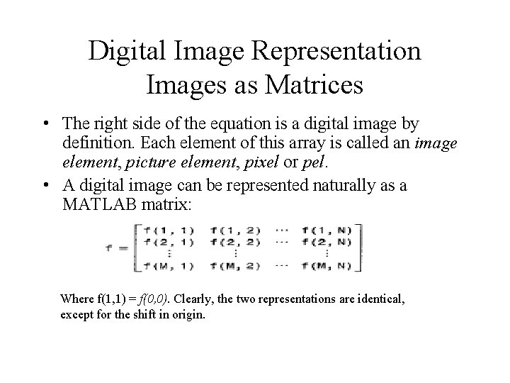
Digital Image Representation Images as Matrices • The right side of the equation is a digital image by definition. Each element of this array is called an image element, picture element, pixel or pel. • A digital image can be represented naturally as a MATLAB matrix: Where f(1, 1) = f(0, 0). Clearly, the two representations are identical, except for the shift in origin.

Digital Image Representation Images as Matrices • Important notations: – f(p, q) denotes the element located in row p and column q. • Ex: f(2, 5) resides in the second row and fifth column – We use the letters M and N, respectively to denote the number of rows and columns in a matrix. – 1 x N matrix, is called a row vector, whereas as M x 1 matrix is called a column vector. – 1 x 1 matrix is a scalar. • Matrices in MATLAB are stored in variables with names such as A, a, RGB, real_array and so on. Variables must begin with a letter and contain only letters, numerals and underscores.

Reading Images • Images are read into MATLAB environment using function imread, whose syntax is: imread (‘filename’) filename: is a string containing the complete name of the image file (including and applicable extension) Ex: >> f = imread (‘xray. jpg’)

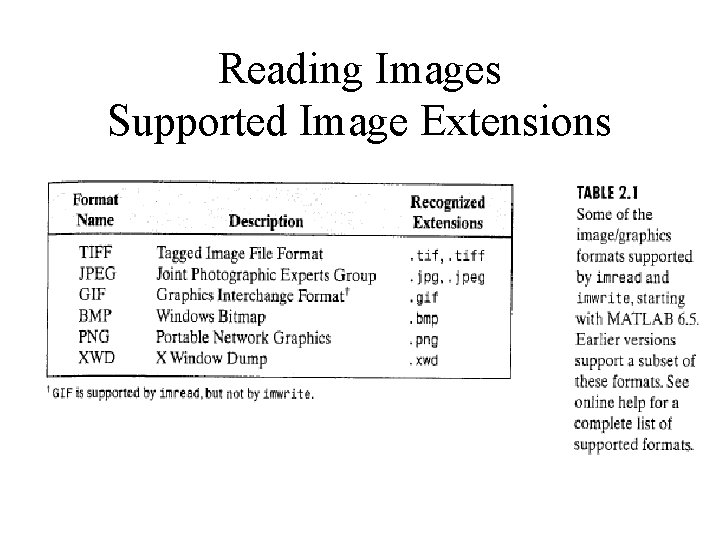
Reading Images Supported Image Extensions

Reading Images Tip - Semicolon • The use of Semicolon: – When using a Semicolon at the end of a command it will stop the output from appearing, and creates directly another prompt symbol (>>) – While, when not using a semicolon, the output will be displayed directly in the Command window (Hint: the output of imread function, is the matrix of the read image)

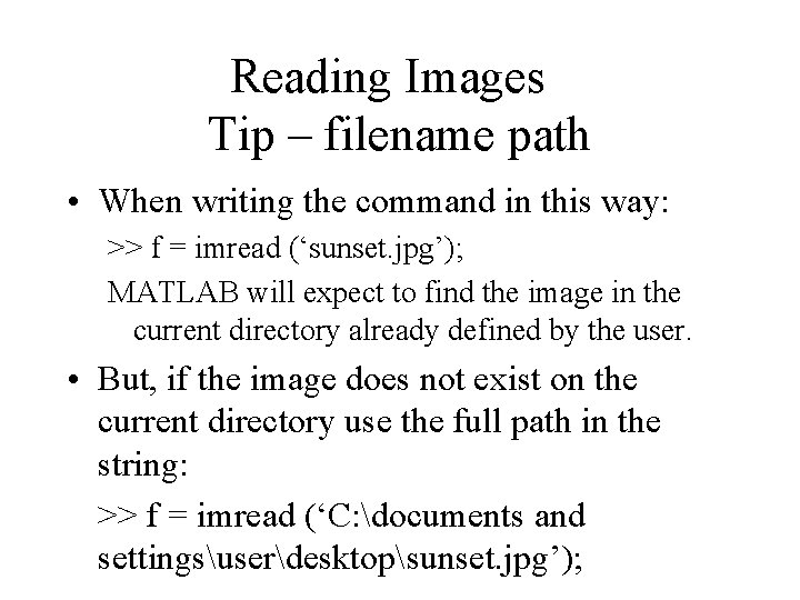
Reading Images Tip – filename path • When writing the command in this way: >> f = imread (‘sunset. jpg’); MATLAB will expect to find the image in the current directory already defined by the user. • But, if the image does not exist on the current directory use the full path in the string: >> f = imread (‘C: documents and settingsuserdesktopsunset. jpg’);

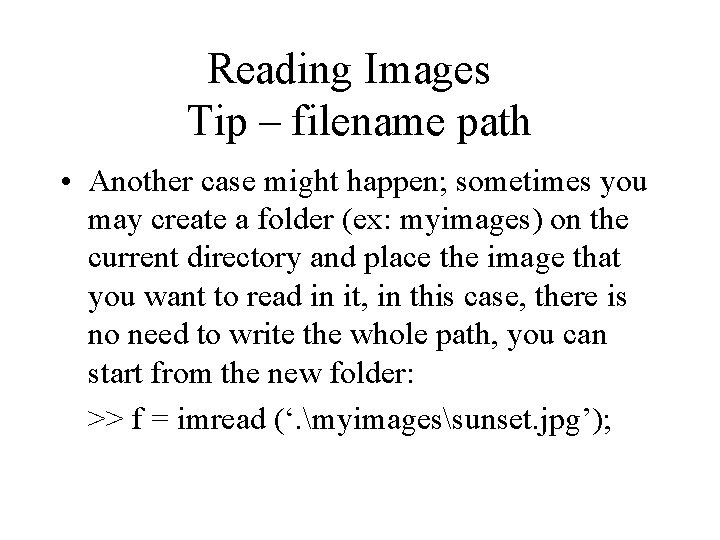
Reading Images Tip – filename path • Another case might happen; sometimes you may create a folder (ex: myimages) on the current directory and place the image that you want to read in it, in this case, there is no need to write the whole path, you can start from the new folder: >> f = imread (‘. myimagessunset. jpg’);

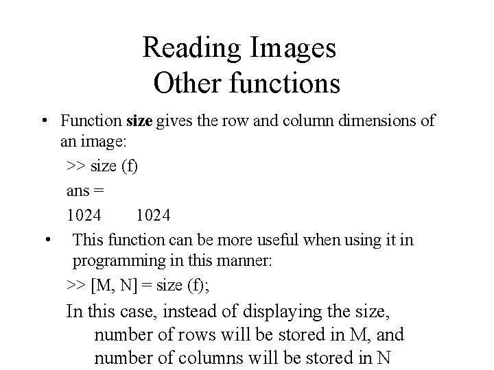
Reading Images Other functions • Function size gives the row and column dimensions of an image: >> size (f) ans = 1024 • This function can be more useful when using it in programming in this manner: >> [M, N] = size (f); In this case, instead of displaying the size, number of rows will be stored in M, and number of columns will be stored in N

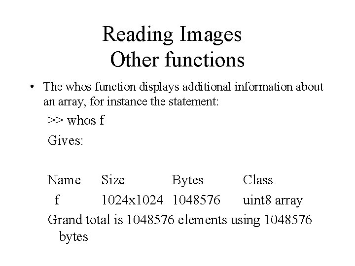
Reading Images Other functions • The whos function displays additional information about an array, for instance the statement: >> whos f Gives: Name Size Bytes Class f 1024 x 1024 1048576 uint 8 array Grand total is 1048576 elements using 1048576 bytes

Displaying Images • Images are displayed on MATLAB desktop using function imshow, which has the basic syntax: imshow (f (: , C), G) where f is an image array, and G is the number of grey levels used to display it. If G is omitted, it defaults to 256 grey levels, C is the color to change used either (1, 2 or 3)

Displaying Images • Using the syntax imshow (f (: , C), [low high]) Displays as black all values less than or equal to low, and as white all values greater than or equal to high. Ex: imshow (f(: , 2), [20 25])

Displaying Images • Finally, the syntax imshow (f(: , 2), [ ]) Sets variable low to the minimum value of array f, and high to the maximum value.

Displaying Images • Function pixval is used frequently to display the intensity values of individual pixels interactively • This function displays a cursor overlaid on an image. As the cursor is moved over the image with the mouse, the coordinates of the cursor position and the corresponding intensity values are shown on a display that appears below the Figure window. • When working with color images, the coordinates as well as the red, green and blue components are displayed.

Displaying Images • If another image, g, is displayed using imshow, MATLAB replaces the image in the screen with the new image. To keep the first image and output a second image, we use function figure as follows: >> figure, imshow (g) • Using the statement: >> imshow(f), figure, imshow(g) displays both images. Note that more than one command can be written on a line, as long as different commands are properly delimited by commas or semicolons.

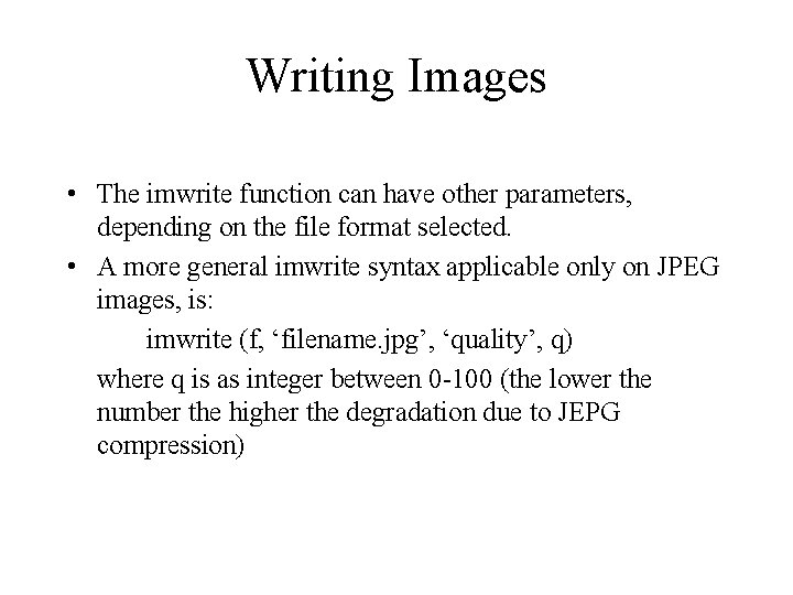
Writing Images • Images are written to disk using function imwrite, which has the following basic syntax: imwrite (f, ‘filename’) • With this syntax, the string contained in filename must include a recognized format extension (mentioned earlier). Alternatively, the desired format can be specified explicitly with a third input argument. For example, the following two commands are the same: >> imwrite (f, ‘file 1. tif’) >> imwrite(f, ‘file 1’, ‘tif’) • If filename contains no path information, then imwrite saves the file in the current working directory.

Writing Images • The imwrite function can have other parameters, depending on the file format selected. • A more general imwrite syntax applicable only on JPEG images, is: imwrite (f, ‘filename. jpg’, ‘quality’, q) where q is as integer between 0 -100 (the lower the number the higher the degradation due to JEPG compression)

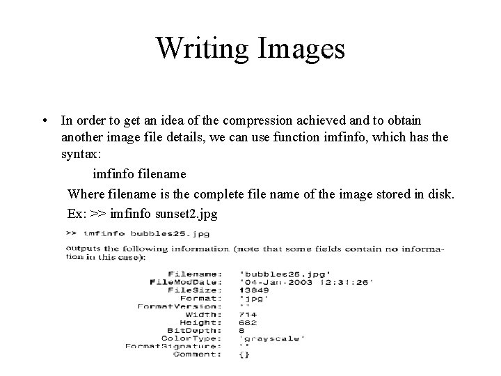
Writing Images • In order to get an idea of the compression achieved and to obtain another image file details, we can use function imfinfo, which has the syntax: imfinfo filename Where filename is the complete file name of the image stored in disk. Ex: >> imfinfo sunset 2. jpg

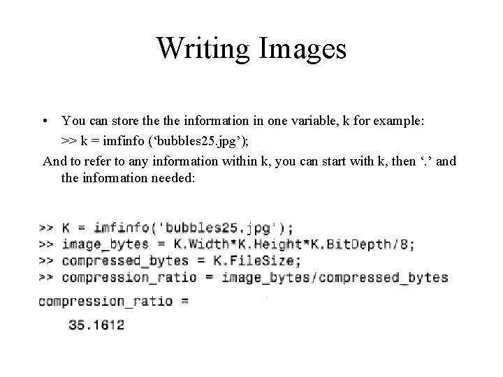
Writing Images • You can store the information in one variable, k for example: >> k = imfinfo (‘bubbles 25. jpg’); And to refer to any information within k, you can start with k, then ‘. ’ and the information needed:

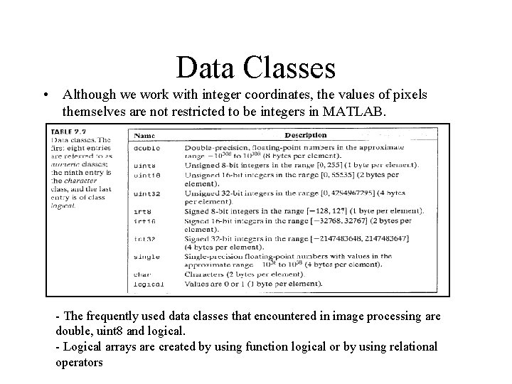
Data Classes • Although we work with integer coordinates, the values of pixels themselves are not restricted to be integers in MATLAB. - The frequently used data classes that encountered in image processing are double, uint 8 and logical. - Logical arrays are created by using function logical or by using relational operators

Image Types • The toolbox supports four types of images: – Intensity Images – Binary Images – Indexed Images – RGB Images

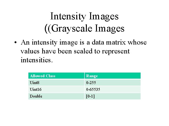
Intensity Images ((Grayscale Images • An intensity image is a data matrix whose values have been scaled to represent intensities. Allowed Class Range Uint 8 0 -255 Uint 16 0 -65535 Double [0 -1]

Binary Images • Logical array containing only 0 s and 1 s, interpreted as black and white, respectively. • If the array contains 0 s and 1 s whose values are of data class different from logical (for example uint 8), it is not considered a binary image in MATLAB.

Binary Images • To convert a numeric array to binary, we use function logical: >> A = [0 1 1 1]; >> B = logical (A); • If A contains other than 0 s and 1 s, the logical function converts all nonzero values to logical 1 s. >> A = [0 3 1 0 4 0]; >> B = logical (B); >> B 011010

Binary Images • By using relational and logical operations, we can also create a logical array • To test if an array is logical, we use islogical function: >> islogical (A); Returns 1, if A is logical, and 0, otherwise • Logical arrays can be converted into numerical arrays using the data class conversion functions.

Indexed Images • An index image consists of an array and a color map matrix. • The pixel values in an array are direct indices into a color map.

RGB Images • Also called, true color images, require a three – dimensional array, (M x N x 3)of class uint 8, uint 16, single or double, whose pixel values specify intensity values. • Unlike an indexed image, however, these intensity values are stored directly in the image array, not indirectly in a color map. • M and N are the numbers of rows and columns of pixels in the image, and the third dimension consists of three planes, containing red, green and blue intensity values.

Converting between Data Classes • The general syntax is B = data_class_name (A) Where data_class_name is one of the names defined in the previous lecture for Data Classes Ex: B = double (A) D = uint 8(C) Note: Take into consideration the data range for each of the data classes before conversion