Digital Image Processing 10302020 Digital Image Processing 1

Digital Image Processing 10/30/2020 Digital Image Processing 1

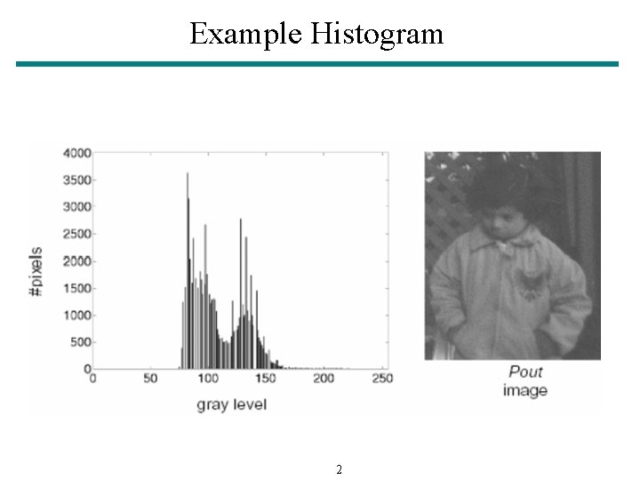
Example Histogram 2

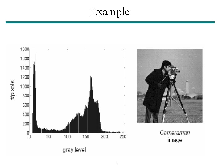
Example 3

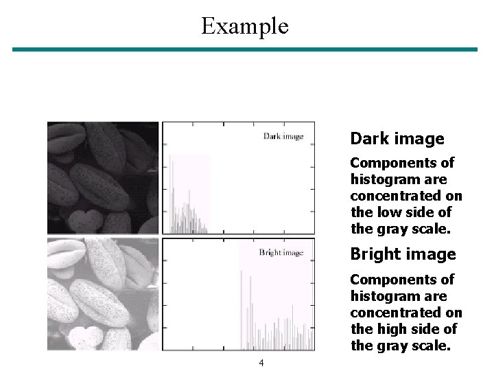
Example Dark image Components of histogram are concentrated on the low side of the gray scale. Bright image Components of histogram are concentrated on the high side of the gray scale. 4

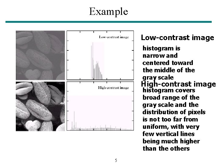
Example Low-contrast image histogram is narrow and centered toward the middle of the gray scale High-contrast image histogram covers broad range of the gray scale and the distribution of pixels is not too far from uniform, with very few vertical lines being much higher than the others 5

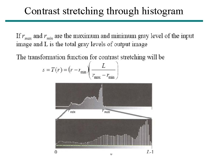
Contrast stretching through histogram 6

7

Digital Image Processing Lecture 9: Image Enhancement in Spatial Domain Spatial Filtering: Order statistic filtering and Image Sharpening 10/30/2020 Digital Image Processing 8

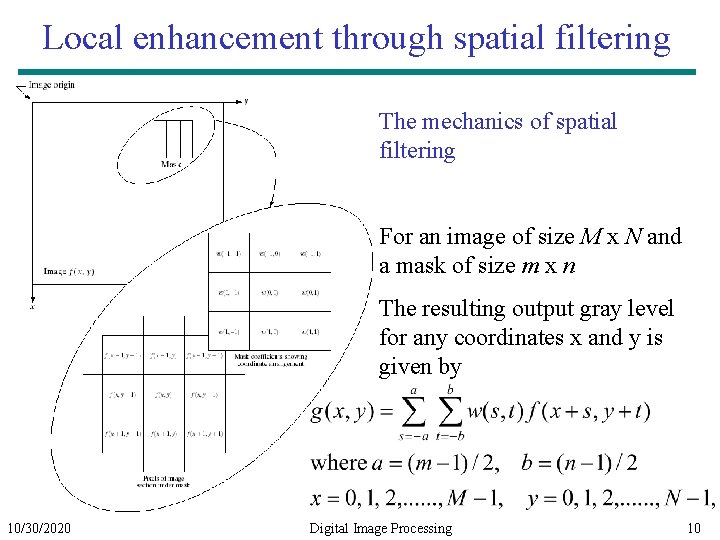
Local enhancement through spatial filtering § The output intensity value at (x, y) depends not only on the input intensity value at (x, y) but also on the specified number of neighboring intensity values around (x, y) § Spatial masks (also called window, filter, kernel, template) are used and convolved over the entire image for local enhancement (spatial filtering) § The size of the masks determines the number of neighboring pixels which influence the output value at (x, y) § The values (coefficients) of the mask determine the nature and properties of enhancing technique 10/30/2020 Digital Image Processing 9

Local enhancement through spatial filtering The mechanics of spatial filtering For an image of size M x N and a mask of size m x n The resulting output gray level for any coordinates x and y is given by 10/30/2020 Digital Image Processing 10

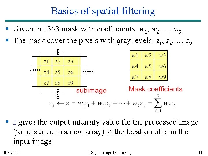
Basics of spatial filtering § Given the 3× 3 mask with coefficients: w 1, w 2, …, w 9 § The mask cover the pixels with gray levels: z 1, z 2, …, z 9 § z gives the output intensity value for the processed image (to be stored in a new array) at the location of z 5 in the input image 10/30/2020 Digital Image Processing 11

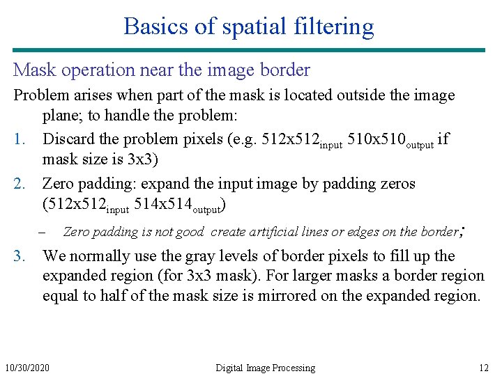
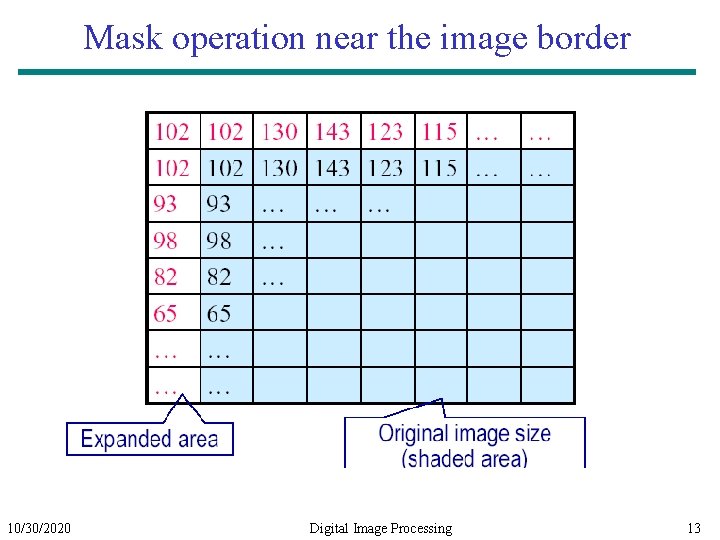
Basics of spatial filtering Mask operation near the image border Problem arises when part of the mask is located outside the image plane; to handle the problem: 1. Discard the problem pixels (e. g. 512 x 512 input 510 x 510 output if mask size is 3 x 3) 2. Zero padding: expand the input image by padding zeros (512 x 512 input 514 x 514 output) – Zero padding is not good create artificial lines or edges on the border; 3. We normally use the gray levels of border pixels to fill up the expanded region (for 3 x 3 mask). For larger masks a border region equal to half of the mask size is mirrored on the expanded region. 10/30/2020 Digital Image Processing 12

Mask operation near the image border 10/30/2020 Digital Image Processing 13

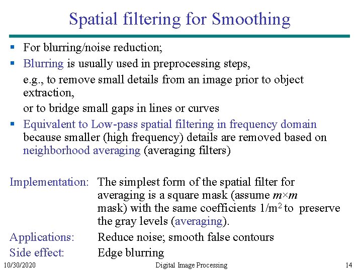
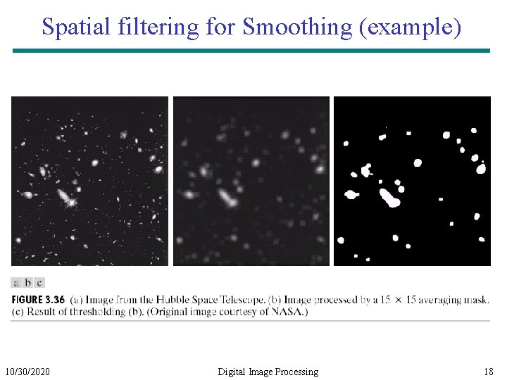
Spatial filtering for Smoothing § For blurring/noise reduction; § Blurring is usually used in preprocessing steps, e. g. , to remove small details from an image prior to object extraction, or to bridge small gaps in lines or curves § Equivalent to Low-pass spatial filtering in frequency domain because smaller (high frequency) details are removed based on neighborhood averaging (averaging filters) Implementation: The simplest form of the spatial filter for averaging is a square mask (assume m×m mask) with the same coefficients 1/m 2 to preserve the gray levels (averaging). Applications: Reduce noise; smooth false contours Side effect: Edge blurring 10/30/2020 Digital Image Processing 14

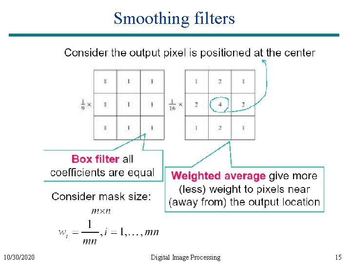
Smoothing filters 10/30/2020 Digital Image Processing 15

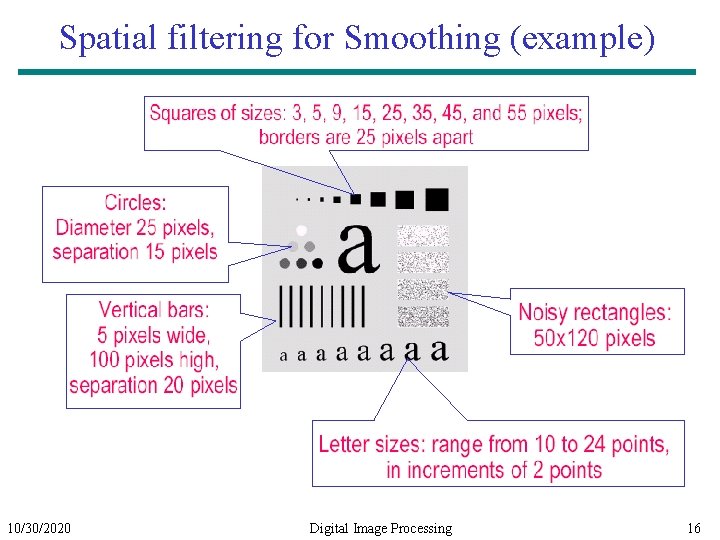
Spatial filtering for Smoothing (example) 10/30/2020 Digital Image Processing 16

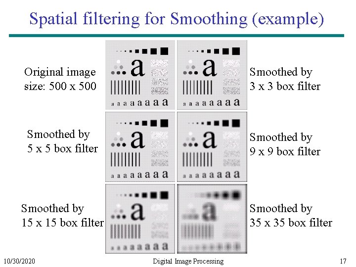
Spatial filtering for Smoothing (example) Original image size: 500 x 500 Smoothed by 3 x 3 box filter Smoothed by 5 x 5 box filter Smoothed by 9 x 9 box filter Smoothed by 15 x 15 box filter 10/30/2020 Smoothed by 35 x 35 box filter Digital Image Processing 17

Spatial filtering for Smoothing (example) 10/30/2020 Digital Image Processing 18

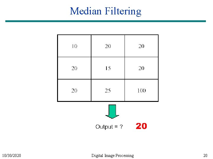
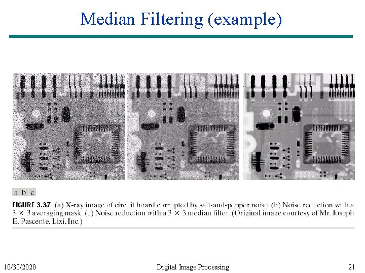
Order-statistics filtering § Nonlinear spatial filters § Output is based on order of gray levels in the masked area (sub-image) § Examples: Median filtering, Max & Min filtering Median filtering § Assigns the mid value of all the gray levels in the mask to the center of mask; § Particularly effective when – the noise pattern consists of strong, spiky components (impulse noise, salt-and-pepper – edges are to be preserved – Force points with distinct gray levels to be more like their neighbors 10/30/2020 Digital Image Processing 19

Median Filtering 10/30/2020 Digital Image Processing 20

Median Filtering (example) 10/30/2020 Digital Image Processing 21

Spatial filtering for image sharpening Background: Applications: to highlight fine detail in an image or to enhance blurred detail electronic printing, medical imaging, industrial inspection, autonomous target detection (smart weapons). . . Foundation: § Blurring/smoothing is performed by spatial averaging (equivalent to integration) § Sharpening is performed by noting only the gray level changes in the image that is the differentiation 10/30/2020 Digital Image Processing 22

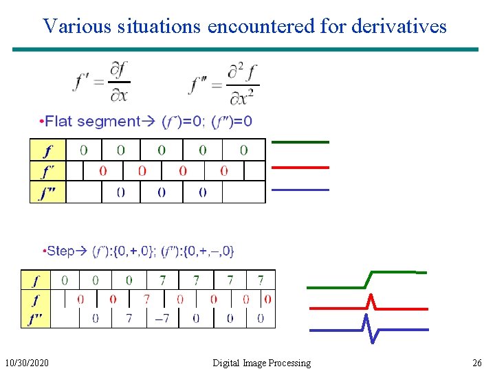
Spatial filtering for image sharpening Operation of Image Differentiation § Enhance edges and discontinuities (magnitude of output gray level >>0) § De-emphasize areas with slowly varying gray-level values (output gray level: 0) Mathematical Basis of Filtering for Image Sharpening § First-order and second-order derivatives § Approximation in discrete-space domain § Implementation by mask filtering 10/30/2020 Digital Image Processing 23

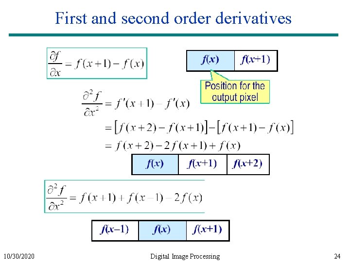
First and second order derivatives 10/30/2020 Digital Image Processing 24

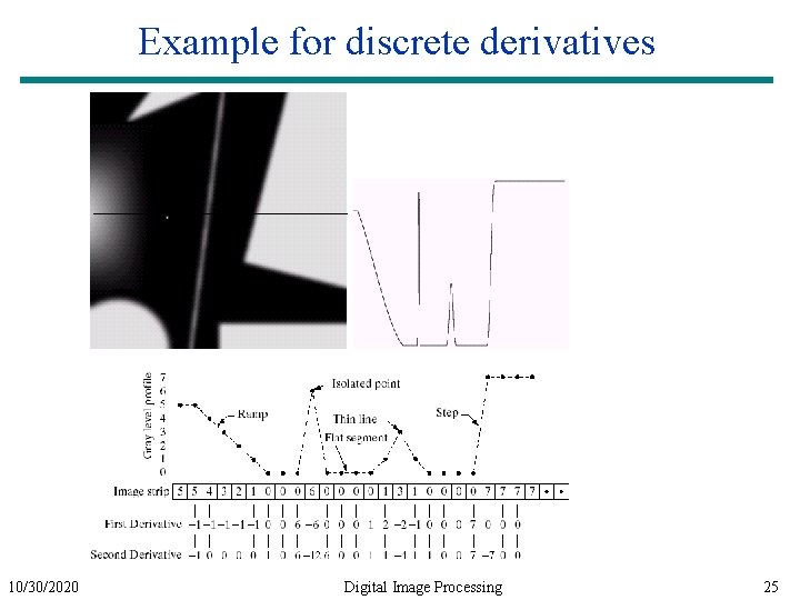
Example for discrete derivatives 10/30/2020 Digital Image Processing 25

Various situations encountered for derivatives 10/30/2020 Digital Image Processing 26

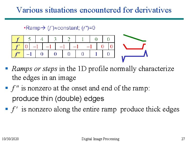
Various situations encountered for derivatives § Ramps or steps in the 1 D profile normally characterize the edges in an image § f ″ is nonzero at the onset and end of the ramp: produce thin (double) edges § f ′ is nonzero along the entire ramp produce thick edges 10/30/2020 Digital Image Processing 27

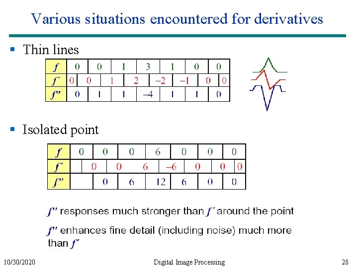
Various situations encountered for derivatives § Thin lines § Isolated point 10/30/2020 Digital Image Processing 28

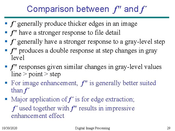
Comparison between f" and f´ § § f´ generally produce thicker edges in an image f" have a stronger response to file detail f´ generally have a stronger response to a gray-level step f" produces a double response at step changes in gray level § f" responses given similar changes in gray-level values line > point > step § For image enhancement, f" is generally better suited than f´ § Major application of f´ is for edge extraction; f´ used together with f" results in impressive enhancement effect 10/30/2020 Digital Image Processing 29

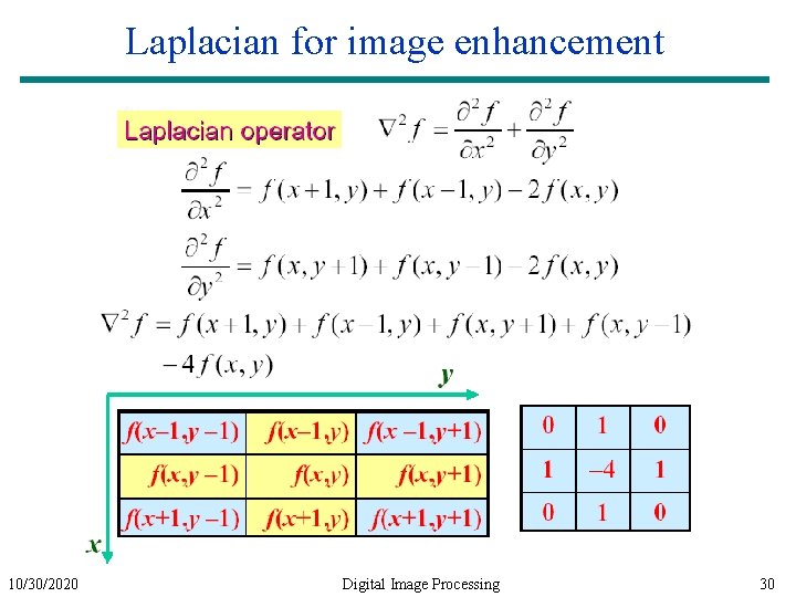
Laplacian for image enhancement 10/30/2020 Digital Image Processing 30

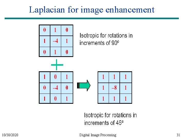
Laplacian for image enhancement 10/30/2020 Digital Image Processing 31

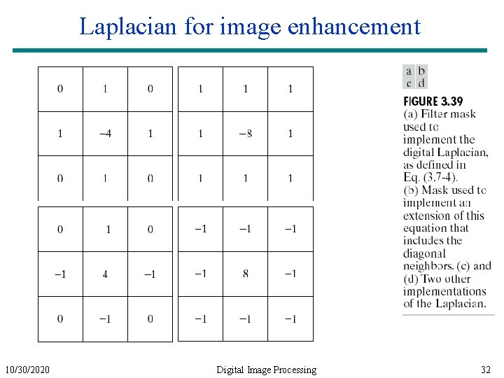
Laplacian for image enhancement 10/30/2020 Digital Image Processing 32

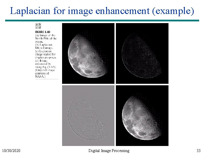
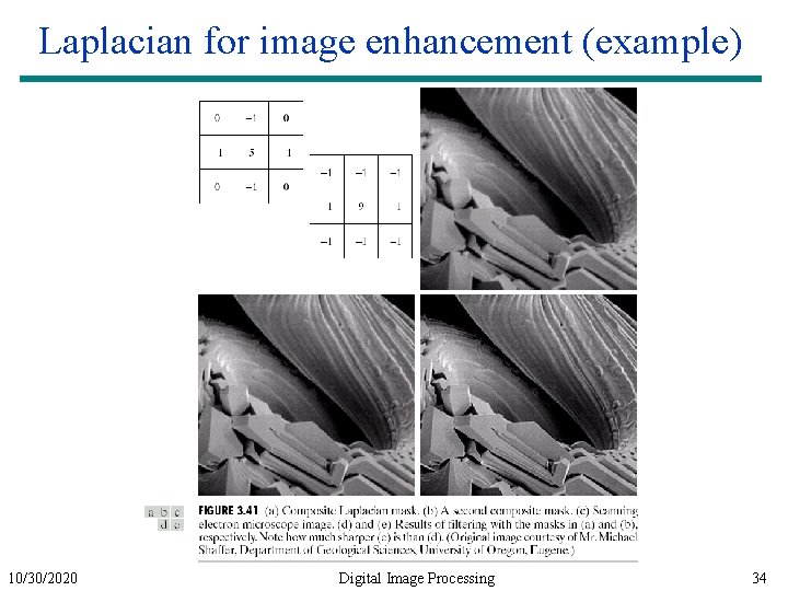
Laplacian for image enhancement (example) 10/30/2020 Digital Image Processing 33

Laplacian for image enhancement (example) 10/30/2020 Digital Image Processing 34