Lecture z Chapter 10 Image Segmentation Segmentation approaches

Lecture z Chapter 10: Image Segmentation

Segmentation approaches 1) Gradient based: How different are pixels? 2) Thresholding: Converts grey-level images to binary so that 1 represents object and 0 the background. 3) Region based segmentation: Looks at similarity between adjacent pixels.

(3) Region based segmentation • Separates the entire region R over which the image is defined into disjoint partitions R 1, R 2, …, Rn. • Each Ri is connected and satisfies some condition P(Ri), whereas (Ri U Rj) does not satisfy the condition.

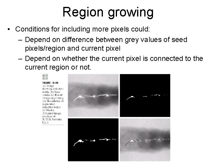
Region growing • Starts with some pixels and grows them into regions based on conditions, a. k. a seed points. • Selecting starting pixels could be done manually or according to some priori knowledge about the problem. • Region growing continues till eithere are no more pixels that can be added or till some stopping criteria is met.

Region growing • Conditions for including more pixels could: – Depend on difference between grey values of seed pixels/region and current pixel – Depend on whether the current pixel is connected to the current region or not.

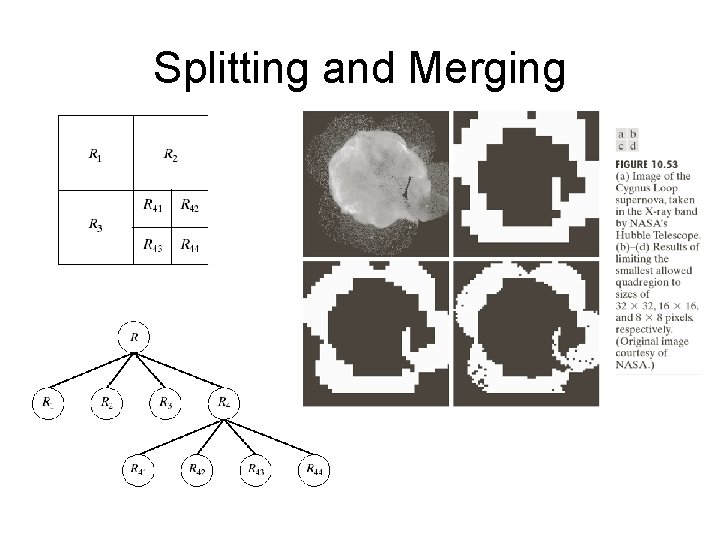
Region Splitting and Merging • Start with the entire image region. • Divide into 4 quadrants if the region does not satisfy certain condition. • Continue dividing the sub-regions into 4 subquadrants till they satisfy the defined condition – Quadtree representation. • Can end up with too many regions. • Merge adjacent regions Ri, Rj if Ri U Rj satisfy the condition. • Stop when no further splitting or merging is possible.

Splitting and Merging

Watershed segmentation Some slides from Eli Turkel’s presentation on Watershed Segmentation, Tel Aviv University

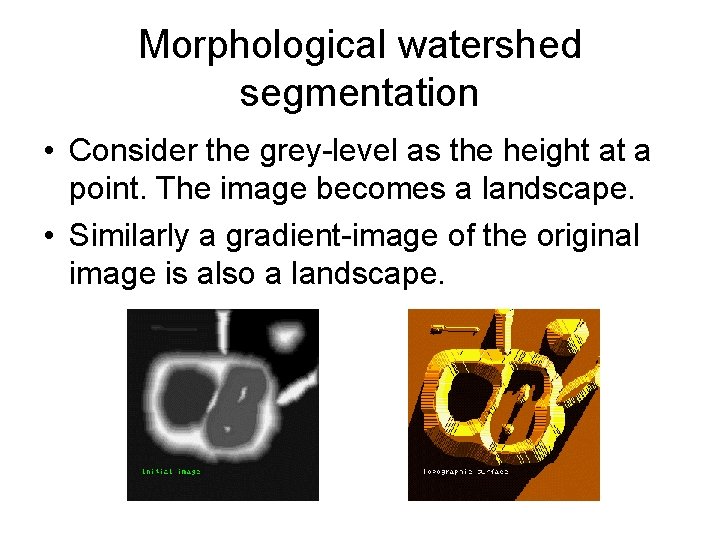
Morphological watershed segmentation • Consider the grey-level as the height at a point. The image becomes a landscape. • Similarly a gradient-image of the original image is also a landscape.

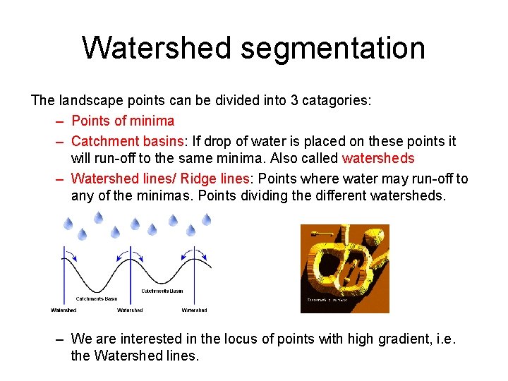
Watershed segmentation The landscape points can be divided into 3 catagories: – Points of minima – Catchment basins: If drop of water is placed on these points it will run-off to the same minima. Also called watersheds – Watershed lines/ Ridge lines: Points where water may run-off to any of the minimas. Points dividing the different watersheds. – We are interested in the locus of points with high gradient, i. e. the Watershed lines.

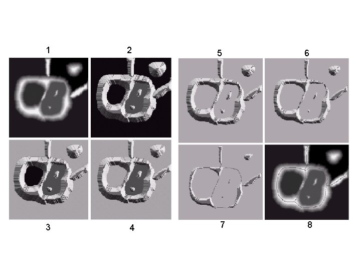
Basic algorithm • • • The 3 D topography is flooded from below gradually (Iterative procedure) When the rising water in distinct catchment basins is about to merge, a dam is built to prevent the merging Finally only the dams would be visible which are exactly the set of points we want.

1 3 2 4 5 7 6 8

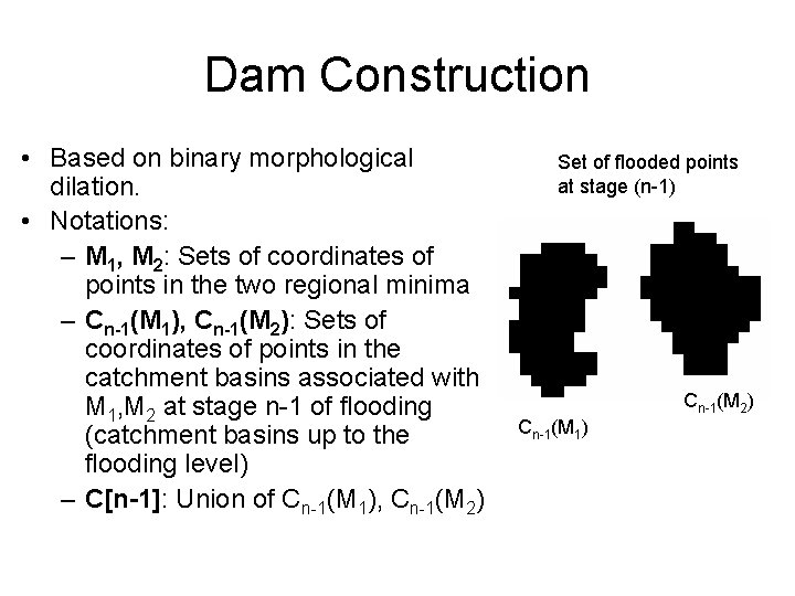
Dam Construction • Based on binary morphological dilation. • Notations: – M 1, M 2: Sets of coordinates of points in the two regional minima – Cn-1(M 1), Cn-1(M 2): Sets of coordinates of points in the catchment basins associated with M 1, M 2 at stage n-1 of flooding (catchment basins up to the flooding level) – C[n-1]: Union of Cn-1(M 1), Cn-1(M 2) Set of flooded points at stage (n-1) Cn-1(M 2) Cn-1(M 1)

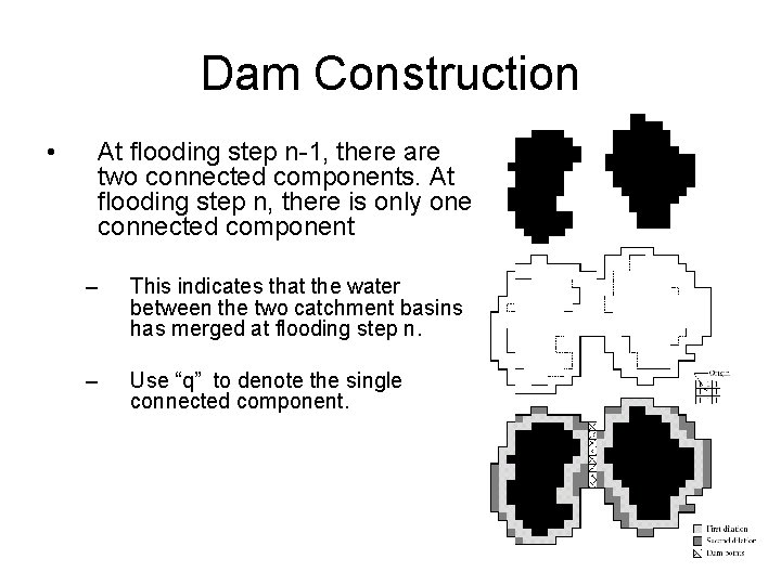
Dam Construction • At flooding step n-1, there are two connected components. At flooding step n, there is only one connected component – This indicates that the water between the two catchment basins has merged at flooding step n. – Use “q” to denote the single connected component.

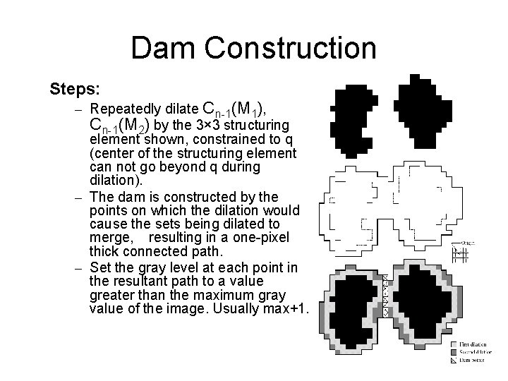
Dam Construction Steps: – Repeatedly dilate Cn-1(M 1), Cn-1(M 2) by the 3× 3 structuring element shown, constrained to q (center of the structuring element can not go beyond q during dilation). – The dam is constructed by the points on which the dilation would cause the sets being dilated to merge, resulting in a one-pixel thick connected path. – Set the gray level at each point in the resultant path to a value greater than the maximum gray value of the image. Usually max+1.

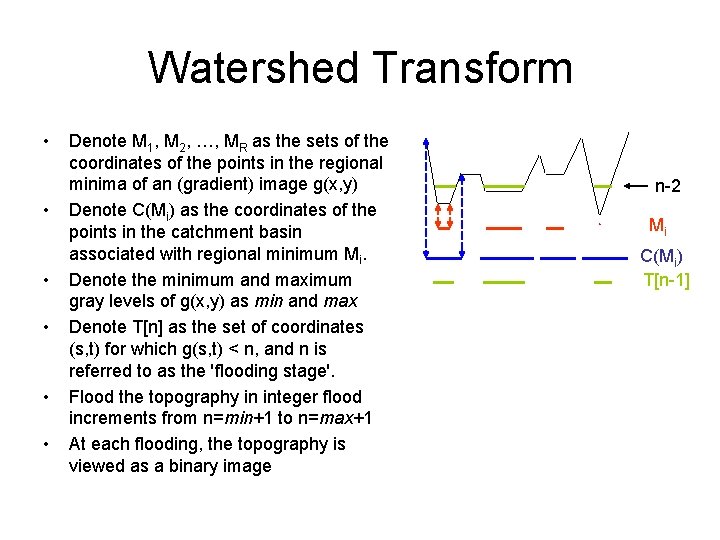
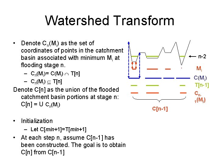
Watershed Transform • • • Denote M 1, M 2, …, MR as the sets of the coordinates of the points in the regional minima of an (gradient) image g(x, y) Denote C(Mi) as the coordinates of the points in the catchment basin associated with regional minimum Mi. Denote the minimum and maximum gray levels of g(x, y) as min and max Denote T[n] as the set of coordinates (s, t) for which g(s, t) < n, and n is referred to as the 'flooding stage'. Flood the topography in integer flood increments from n=min+1 to n=max+1 At each flooding, the topography is viewed as a binary image n-2 Mi C(Mi) T[n-1]

Watershed Transform • Denote Cn(Mi) as the set of coordinates of points in the catchment basin associated with minimum Mi at flooding stage n. n-2 Mi – Cn(Mi)= C(Mi) T[n] – Cn(Mi) T[n] Denote C[n] as the union of the flooded catchment basin portions at stage n: C[n] = U Cn(Mi) • Initialization – Let C[min+1]=T[min+1] • At each step n, assume C[n-1] has been constructed. The goal is to obtain C[n] from C[n-1] C(Mi) T[n-1] Cn 1(Mi) C[n-1]

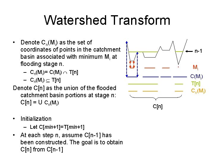
Watershed Transform • Denote Cn(Mi) as the set of coordinates of points in the catchment basin associated with minimum Mi at flooding stage n. n-1 Mi – Cn(Mi)= C(Mi) T[n] – Cn(Mi) T[n] Denote C[n] as the union of the flooded catchment basin portions at stage n: C[n] = U Cn(Mi) • Initialization – Let C[min+1]=T[min+1] • At each step n, assume C[n-1] has been constructed. The goal is to obtain C[n] from C[n-1] C(Mi) T[n] Cn(Mi) C[n]

Watershed Transform Dam • For each connected component q Q[n], there are three possibilities: n-1 (a) q C[n-1] is empty (q 1) • • n-2 A new minimum is encountered q is incorporated into C[n-1] to form C[n] Mi (b) q C[n-1] contains one connected component of C[n-1] (q 2) • C(Mi) T[n-1] Cn-1(Mi) q is incorporated into C[n-1] to form C[n] (c) q C[n-1] contains more than one connected components of C[n-1] (q 3) • A ridge separating two or more catchment basins has been encountered A dam has to be built within q to prevent overflow between the catchment C[n-1] q 3 q 1 basins Repeat the procedure until n=max+1 C[n] T[n] q 2

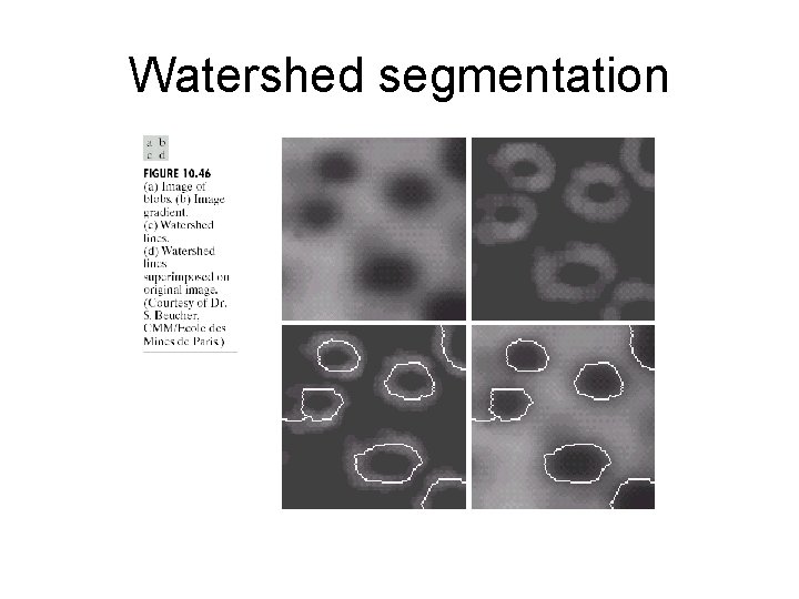
Watershed segmentation

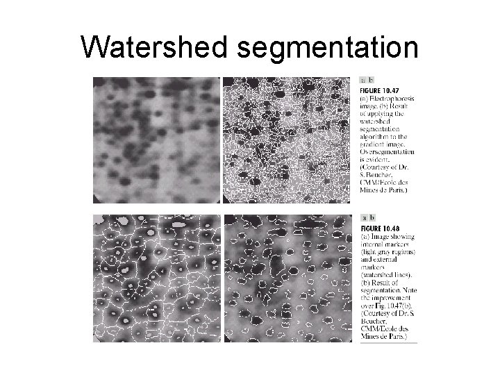
Watershed segmentation

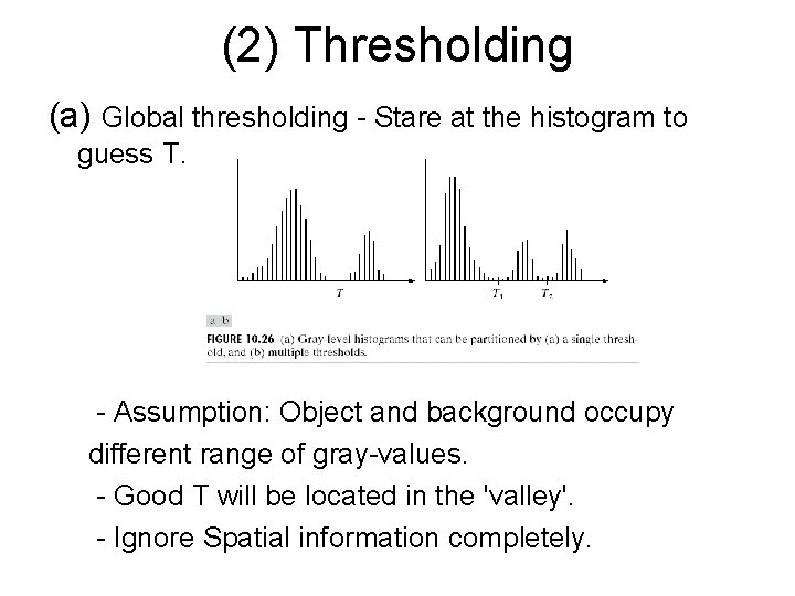
(2) Thresholding (a) Global thresholding - Stare at the histogram to guess T. - Assumption: Object and background occupy different range of gray-values. - Good T will be located in the 'valley'. - Ignore Spatial information completely.

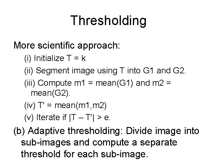
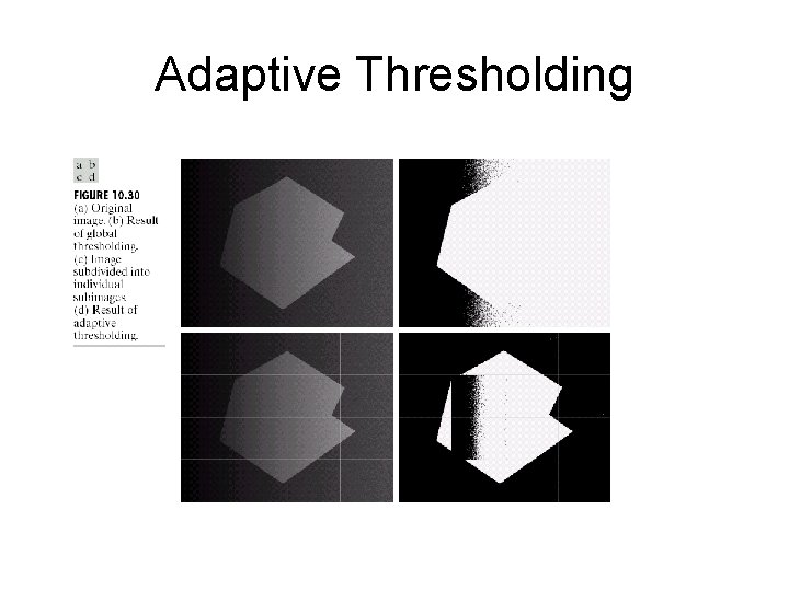
Thresholding More scientific approach: (i) Initialize T = k (ii) Segment image using T into G 1 and G 2. (iii) Compute m 1 = mean(G 1) and m 2 = mean(G 2). (iv) T' = mean(m 1, m 2) (v) Iterate if |T – T'| > e. (b) Adaptive thresholding: Divide image into sub-images and compute a separate threshold for each sub-image.

Adaptive Thresholding

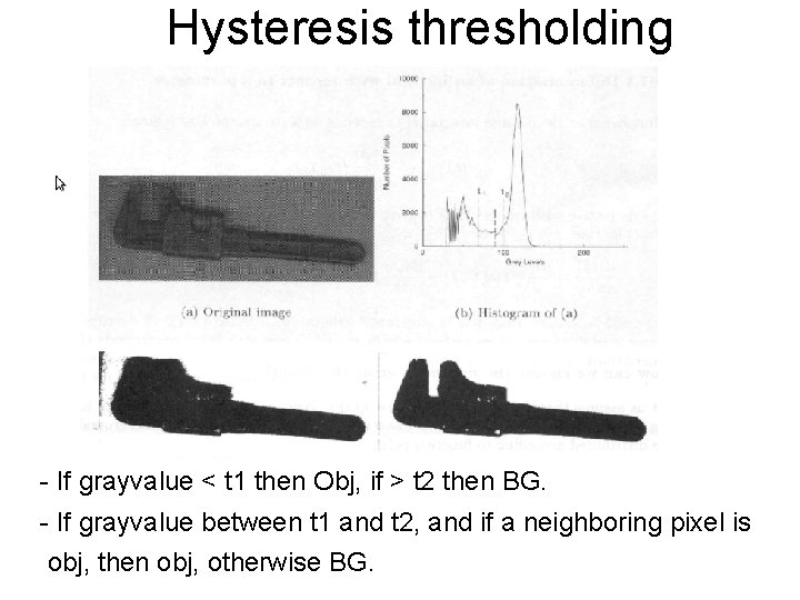
Hysteresis thresholding - If grayvalue < t 1 then Obj, if > t 2 then BG. - If grayvalue between t 1 and t 2, and if a neighboring pixel is obj, then obj, otherwise BG.

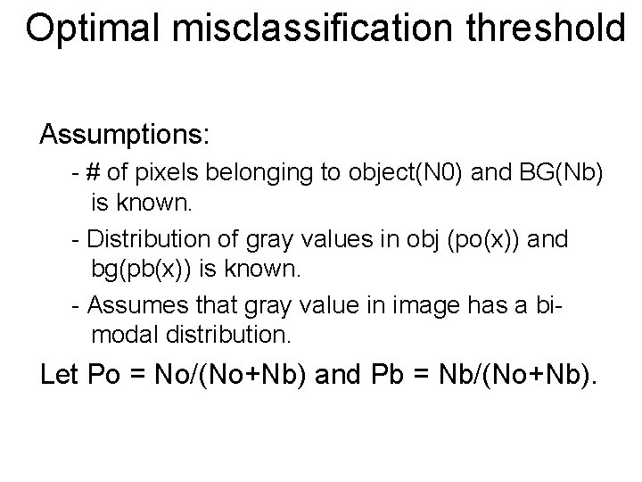
Optimal misclassification threshold Assumptions: - # of pixels belonging to object(N 0) and BG(Nb) is known. - Distribution of gray values in obj (po(x)) and bg(pb(x)) is known. - Assumes that gray value in image has a bimodal distribution. Let Po = No/(No+Nb) and Pb = Nb/(No+Nb).

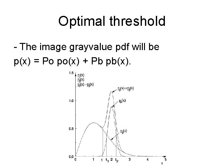
Optimal threshold - The image grayvalue pdf will be p(x) = Po po(x) + Pb pb(x).

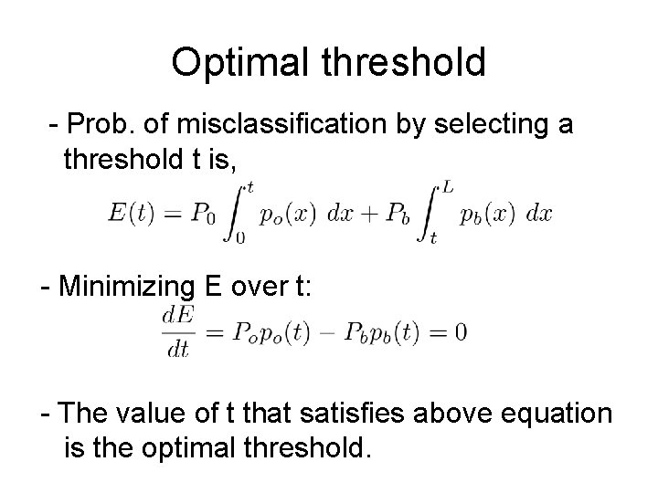
Optimal threshold - Prob. of misclassification by selecting a threshold t is, - Minimizing E over t: - The value of t that satisfies above equation is the optimal threshold.

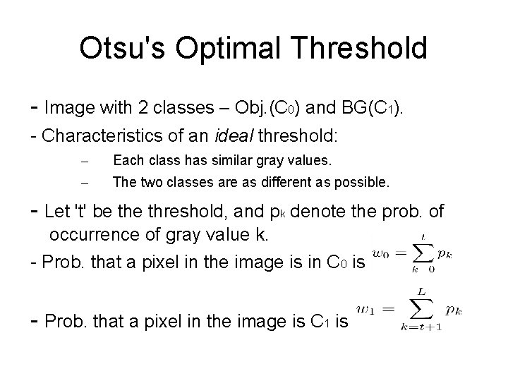
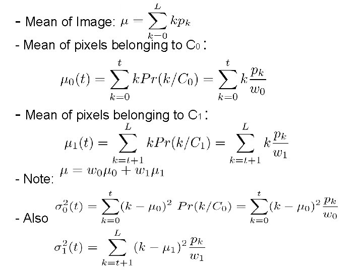
Otsu's Optimal Threshold - Image with 2 classes – Obj. (C 0) and BG(C 1). - Characteristics of an ideal threshold: – Each class has similar gray values. – The two classes are as different as possible. - Let 't' be threshold, and pk denote the prob. of occurrence of gray value k. - Prob. that a pixel in the image is in C 0 is - Prob. that a pixel in the image is C 1 is

- Mean of Image: - Mean of pixels belonging to C 0 : - Mean of pixels belonging to C 1 : - Note: - Also

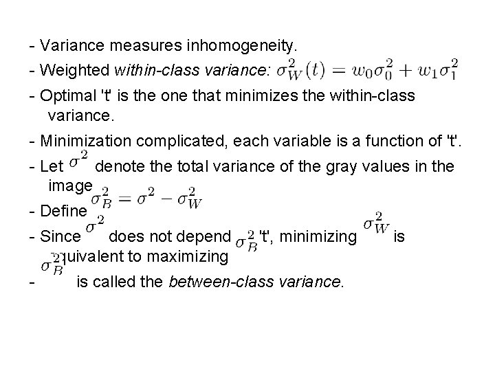
- Variance measures inhomogeneity. - Weighted within-class variance: - Optimal 't' is the one that minimizes the within-class variance. - Minimization complicated, each variable is a function of 't'. - Let denote the total variance of the gray values in the image. - Define - Since does not depend on 't', minimizing equivalent to maximizing - is called the between-class variance. is

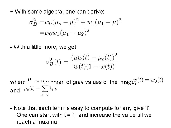
- With some algebra, one can derive: - With a little more, we get where is the mean of gray values of the image, and - Note that each term is easy to compute for any give 't'. One can start with t = 1, and increase the value till we reach a maxima.