Cristina Fernndez Payroll Taxes The Reform Payroll taxes

Cristina Fernández Payroll Taxes

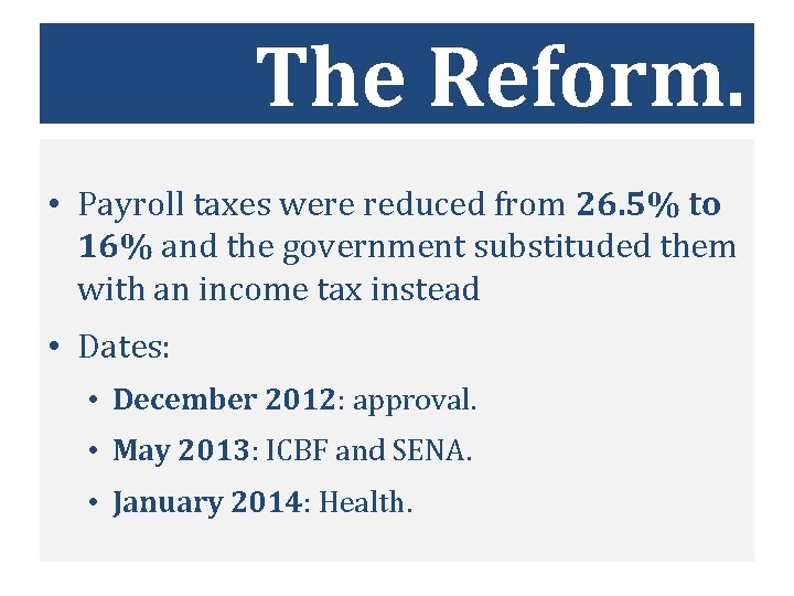
The Reform. • Payroll taxes were reduced from 26. 5% to 16% and the government substituded them with an income tax instead • Dates: • December 2012: approval. • May 2013: ICBF and SENA. • January 2014: Health.

Literature review.

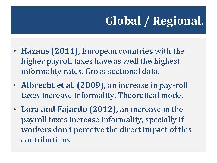
Global / Regional. • Hazans (2011), European countries with the higher payroll taxes have as well the highest informality rates. Cross-sectional data. • Albrecht et al. (2009), an increase in pay-roll taxes increase informality. Theoretical mode. • Lora and Fajardo (2012), an increase in the payroll taxes increase informality, specially if workers don’t perceive the direct impact of this contributions.

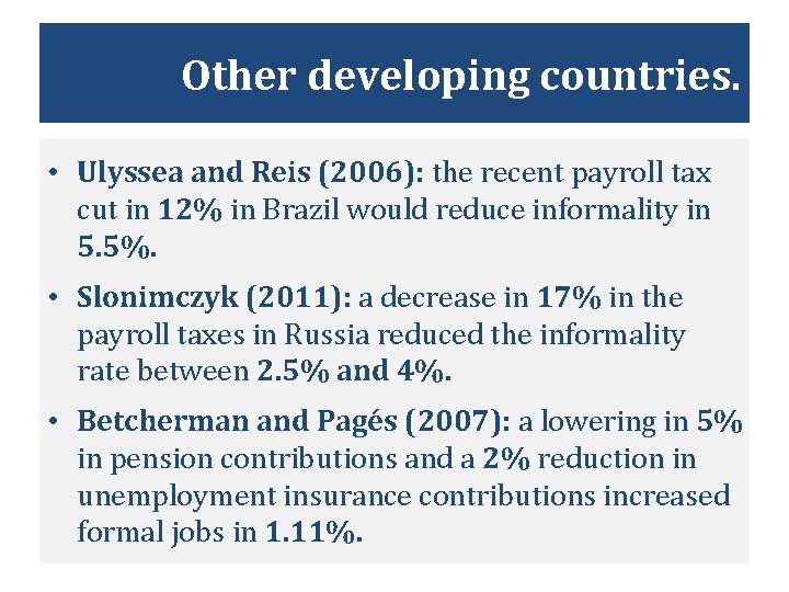
Other developing countries. • Ulyssea and Reis (2006): the recent payroll tax cut in 12% in Brazil would reduce informality in 5. 5%. • Slonimczyk (2011): a decrease in 17% in the payroll taxes in Russia reduced the informality rate between 2. 5% and 4%. • Betcherman and Pagés (2007): a lowering in 5% in pension contributions and a 2% reduction in unemployment insurance contributions increased formal jobs in 1. 11%.

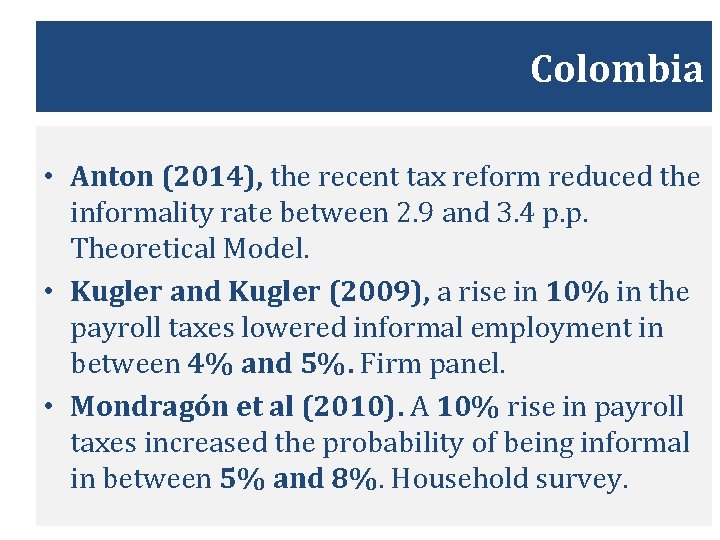
Colombia • Anton (2014), the recent tax reform reduced the informality rate between 2. 9 and 3. 4 p. p. Theoretical Model. • Kugler and Kugler (2009), a rise in 10% in the payroll taxes lowered informal employment in between 4% and 5%. Firm panel. • Mondragón et al (2010). A 10% rise in payroll taxes increased the probability of being informal in between 5% and 8%. Household survey.

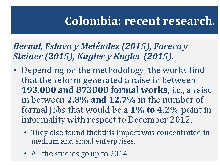
Colombia: recent research. Bernal, Eslava y Meléndez (2015), Forero y Steiner (2015), Kugler y Kugler (2015). • Depending on the methodology, the works find that the reform generated a raise in between 193. 000 and 873000 formal works, i. e. , a raise in between 2. 8% and 12. 7% in the number of formal jobs that would be a 1% to 4. 2% point in informality with respect to December 2012. • They also found that this impact was concentrated in medium and small enterprises. • All the studies go up to 2014.

Informality in Colombia.

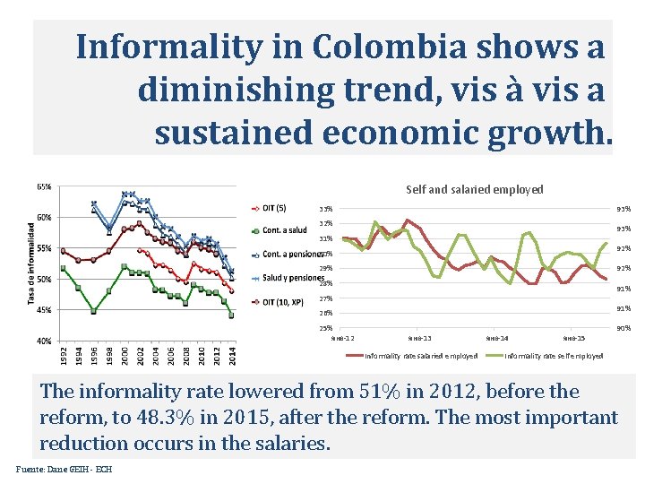
Informality in Colombia shows a diminishing trend, vis à vis a sustained economic growth. Self and salaried employed 33% 93% 32% 93% 31% 92% 30% 29% 92% 28% 91% 27% 91% 26% 25% янв-12 янв-13 Informality rate salaried employed янв-14 янв-15 90% Informality rate self employed The informality rate lowered from 51% in 2012, before the reform, to 48. 3% in 2015, after the reform. The most important reduction occurs in the salaries. Fuente: Dane GEIH - ECH

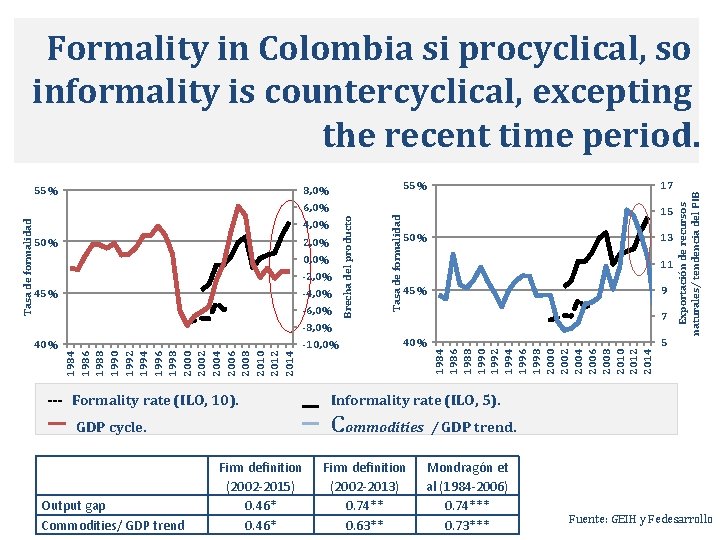
55% 8, 0% 17 2, 0% 0, 0% -2, 0% 45% -4, 0% -6, 0% Tasa de formalidad 50% Brecha del producto 4, 0% 15 50% 13 11 45% 9 7 40% -10, 0% --- Formality rate (ILO, 10). 5 Informality rate (ILO, 5). Commodities / GDP trend. GDP cycle. Output gap Commodities/ GDP trend 40% 1984 1986 1988 1990 1992 1994 1996 1998 2000 2002 2004 2006 2008 2010 2012 2014 -8, 0% 1984 1986 1988 1990 1992 1994 1996 1998 2000 2002 2004 2006 2008 2010 2012 2014 Tasa de formalidad 6, 0% Exportación de recursos naturales/ tendencia del PIB Formality in Colombia si procyclical, so informality is countercyclical, excepting the recent time period. Firm definition (2002 -2015) 0. 46* Firm definition (2002 -2013) 0. 74** 0. 63** Mondragón et al (1984 -2006) 0. 74*** 0. 73*** Fuente: GEIH y Fedesarrollo

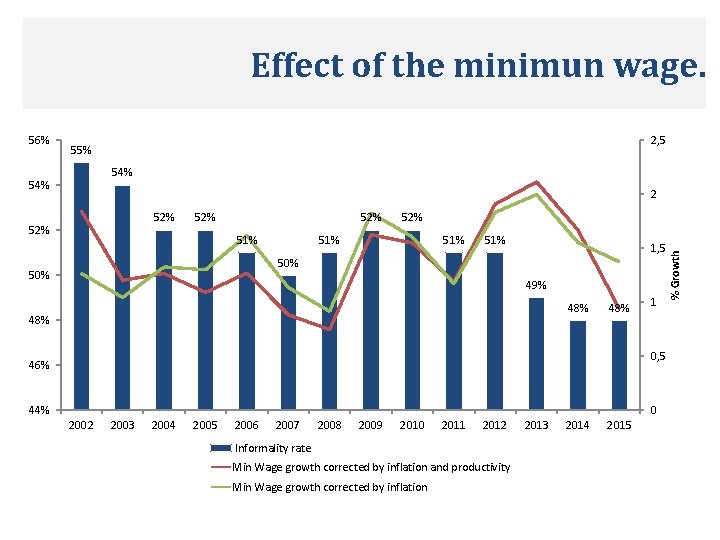
Effect of the minimun wage. 2, 5 55% 54% 2 52% 52% 51% 51% 1, 5 50% 49% 48% 48% 1 0, 5 46% 44% 0 2002 2003 2004 2005 2006 2007 2008 2009 2010 2011 2012 Informality rate Min Wage growth corrected by inflation and productivity Min Wage growth corrected by inflation 2013 2014 2015 % Growth 56%

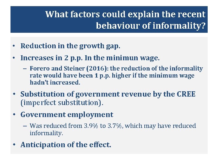
What factors could explain the recent behaviour of informality? • Reduction in the growth gap. • Increases in 2 p. p. In the minimun wage. – Forero and Steiner (2016): the reduction of the informality rate would have been 1 p. p. higher if the minimum wage hadn’t increased. • Substitution of government revenue by the CREE (imperfect substitution). • Government employment – Was reduced from 3. 9% to 3. 7%, which may have reduced informality. • Anticipation of the effect.

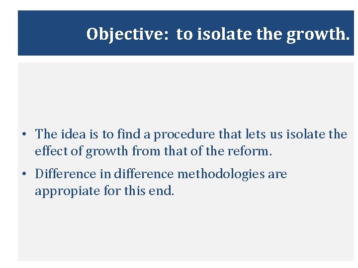
Objective: to isolate the growth. • The idea is to find a procedure that lets us isolate the effect of growth from that of the reform. • Difference in difference methodologies are appropiate for this end.

Differences in differences.

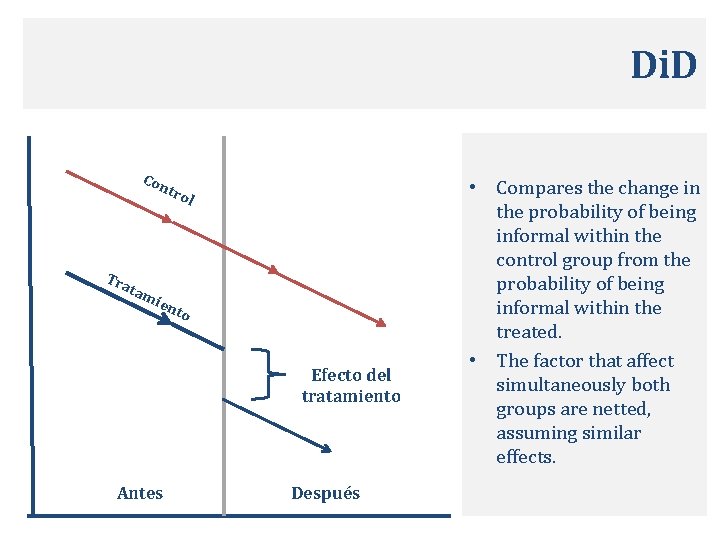
Di. D Con tro Tra tam l ien to Efecto del tratamiento Antes Después • Compares the change in the probability of being informal within the control group from the probability of being informal within the treated. • The factor that affect simultaneously both groups are netted, assuming similar effects.

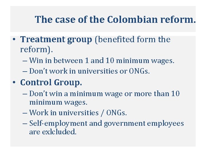
The case of the Colombian reform. • Treatment group (benefited form the reform). – Win in between 1 and 10 minimum wages. – Don’t work in universities or ONGs. • Control Group. – Don’t win a minimum wage or more than 10 minimum wages. – Work in universities / ONGs. – Self-employment and government employees are exlcluded.

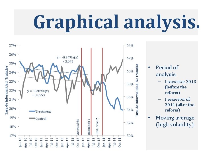
Graphical analysis. • Period of analysis: – I semester 2013 (before the reform) – I semester of 2014 (after the reform) • Moving average (high volatility).

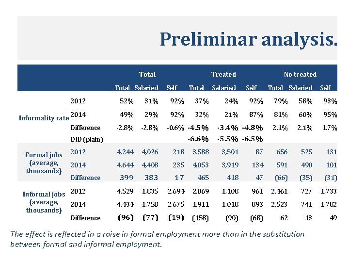
Preliminar analysis. Total Salaried 2012 Informality rate 2014 Difference Treated Self Total Salaried No treated Self Total Salaried Self 52% 31% 92% 37% 24% 92% 79% 58% 93% 49% 29% 92% 32% 21% 87% 81% 60% 95% -2. 8% -3. 4% -4. 8% -5. 5% -6. 5% 2. 1% 1. 7% -0. 6% -4. 5% -6. 6% DID (plain) 2012 4, 244 4, 026 218 3, 588 3, 501 87 656 525 131 2014 4, 644 4, 408 235 4, 053 3, 919 134 591 490 101 Difference 399 383 17 465 418 47 (66) (35) (31) Informal jobs 2012 (average, 2014 thousands) Difference 4, 529 1, 835 2, 694 2, 069 1, 108 961 2, 461 727 1, 733 4, 434 1, 758 2, 675 1, 911 1, 018 893 2, 523 741 1, 782 (96) (77) (19) (158) (90) (68) 62 13 49 Formal jobs (average, thousands) The effect is reflected in a raise in formal employment more than in the substitution between formal and informal employment.

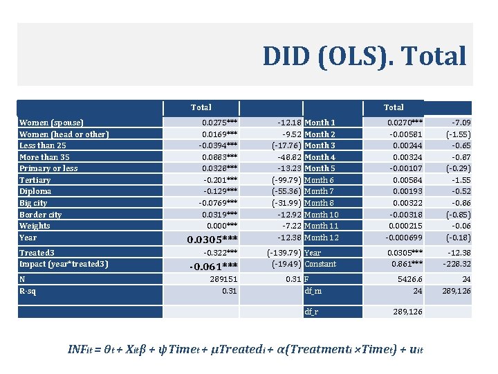
DID (OLS). Total Women (spouse) Women (head or other) Less than 25 More than 35 Primary or less Tertiary Diploma Big city Border city Weights Year Treated 3 Impact (year*treated 3) N R-sq 0. 0275*** 0. 0169*** -0. 0394*** 0. 0883*** 0. 0328*** -0. 201*** -0. 129*** -0. 0769*** 0. 0319*** 0. 000*** 0. 0305*** -0. 322*** -0. 061*** 289151 0. 31 Total -12. 18 -9. 52 (-17. 76) -48. 82 -13. 23 (-99. 79) (-55. 36) (-31. 99) -12. 92 -7. 22 -12. 38 Month 1 Month 2 Month 3 Month 4 Month 5 Month 6 Month 7 Month 8 Month 10 Month 11 Month 12 (-139. 79) Year (-19. 49) Constant 0. 31 F df_m df_r 0. 0270*** -0. 00581 0. 00244 0. 00324 -0. 00107 0. 00584 0. 00193 0. 00322 -0. 00318 0. 000215 -0. 000699 -7. 09 (-1. 55) -0. 65 -0. 87 (-0. 29) -1. 55 -0. 52 -0. 86 (-0. 85) -0. 06 (-0. 18) 0. 0305*** 0. 861*** -12. 38 -228. 32 5426. 6 24 24 289, 126 INFit = θt + Xitβ + ψTimet + μTreatedi + α(Treatmenti ×Timet) + uit

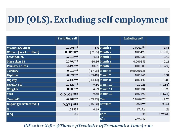
DID (OLS). Excluding self employment Excluding self Women (spouse) Excluding self 0. 0163*** -5. 4 Month 1 0. 0241*** -4. 88 -0. 00678** (-2. 95) Month 2 -0. 00428 (-0. 88) Less than 25 0. 0115*** -4. 32 Month 3 0. 00238 -0. 49 More than 35 0. 0764*** -30. 86 Month 4 0. 000539 -0. 11 Primary or less 0. 0499*** -13. 51 Month 5 -0. 00383 (-0. 79) Tertiary -0. 114*** (-47. 23) Month 6 0. 00000133 0 Diploma -0. 124*** (-39. 40) Month 7 0. 00166 -0. 34 Big city -0. 0429*** (-14. 43) Month 8 0. 00428 -0. 88 Women (head or other) Border city Weights Year Treated 3 R-sq -9. 34 Month 10 -0. 0026 (-0. 54) 0. 000*** -4. 99 Month 11 0. 00134 -0. 28 0. 0406*** -9. 78 Month 12 -0. 00599 (-1. 23) 0. 0406*** -9. 78 0. 653*** -125. 41 1717. 6 24 24 179, 932 -0. 284*** Impact (year*treated 3) N 0. 0324*** -0. 071*** 179957 0. 19 (-85. 73) Year (-15. 08) Constant 0. 19 F df_m df_r 179, 932 INFit = θt + Xitβ + ψTimet + μTreatedi + α(Treatmenti × Timet) + uit

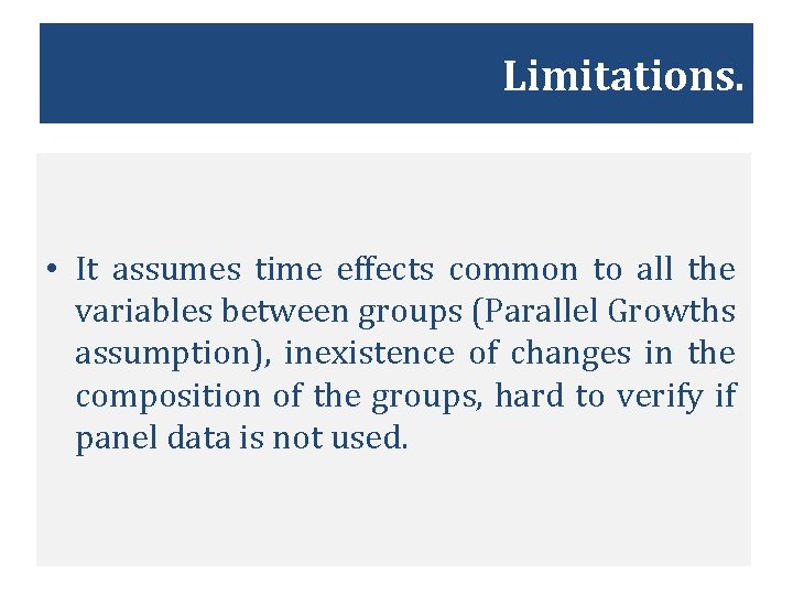
Limitations. • It assumes time effects common to all the variables between groups (Parallel Growths assumption), inexistence of changes in the composition of the groups, hard to verify if panel data is not used.

Matching with differences in differences.

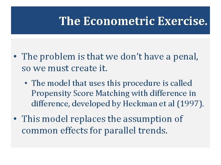
The Econometric Exercise. • The problem is that we don’t have a penal, so we must create it. • The model that uses this procedure is called Propensity Score Matching with difference in difference, developed by Heckman et al (1997). • This model replaces the assumption of common effects for parallel trends.

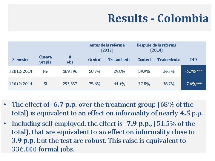
Results - Colombia Antes de la reforma (2012) Después de la reforma (2014) Semester Cuenta propia # obs Control Tratamiento DID I 2012/2014 No 169, 796 58. 3% 29. 8% 59. 9% 24. 7% -6. 7%*** I 2012/2014 Si 293, 337 75. 6% 44. 1% 77. 8% 38. 7% -7. 6%*** • The effect of -6. 7 p. p. over the treatment group (68% of the total) is equivalent to an effect on informality of nearly 4. 5 p. p. • Including self employed, the effect is -7. 9 p. p. , (51. 5% of the total), that are equivalent to an effect on informality close to 3. 9 p. p. but the test are robust. This raise is equivalent to 336. 000 formal jobs.

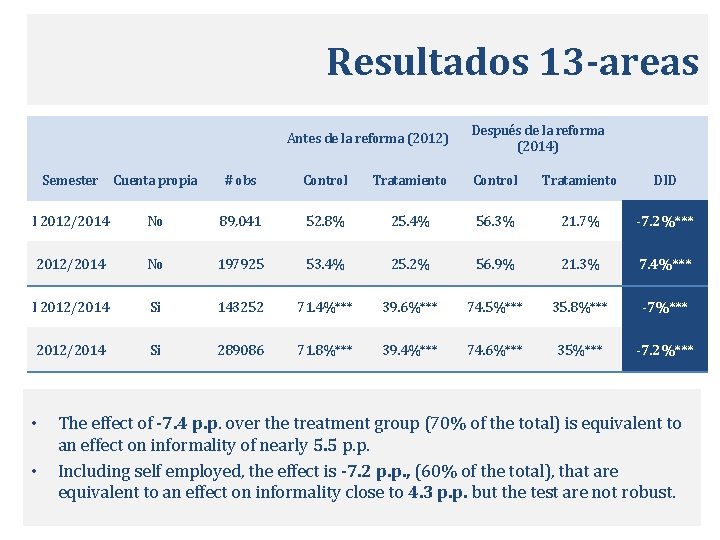
Resultados 13 -areas Antes de la reforma (2012) Después de la reforma (2014) Semester Cuenta propia # obs Control Tratamiento DID I 2012/2014 No 89, 041 52. 8% 25. 4% 56. 3% 21. 7% -7. 2%*** 2012/2014 No 197925 53. 4% 25. 2% 56. 9% 21. 3% 7. 4%*** I 2012/2014 Si 143252 71. 4%*** 39. 6%*** 74. 5%*** 35. 8%*** -7%*** 2012/2014 Si 289086 71. 8%*** 39. 4%*** 74. 6%*** 35%*** -7. 2%*** • • The effect of -7. 4 p. p. over the treatment group (70% of the total) is equivalent to an effect on informality of nearly 5. 5 p. p. Including self employed, the effect is -7. 2 p. p. , (60% of the total), that are equivalent to an effect on informality close to 4. 3 p. p. but the test are not robust.

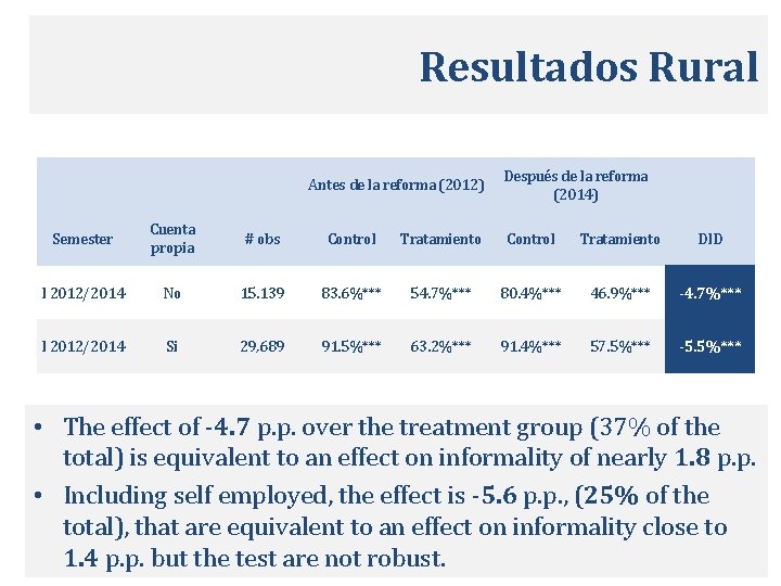
Resultados Rural Antes de la reforma (2012) Después de la reforma (2014) Semester Cuenta propia # obs Control Tratamiento DID I 2012/2014 No 15. 139 83. 6%*** 54. 7%*** 80. 4%*** 46. 9%*** -4. 7%*** I 2012/2014 Si 29, 689 91. 5%*** 63. 2%*** 91. 4%*** 57. 5%*** -5. 5%*** • The effect of -4. 7 p. p. over the treatment group (37% of the total) is equivalent to an effect on informality of nearly 1. 8 p. p. • Including self employed, the effect is -5. 6 p. p. , (25% of the total), that are equivalent to an effect on informality close to 1. 4 p. p. but the test are not robust.

Test (13 areas).

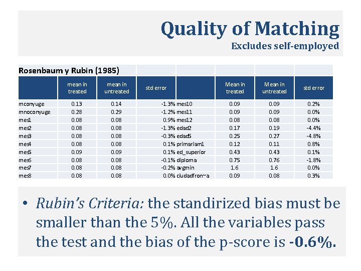
Quality of Matching Excludes self-employed Rosenbaum y Rubin (1985) mconyuge mnoconyuge mes 1 mes 2 mes 3 mes 4 mes 5 mes 6 mes 7 mes 8 mean in treated mean in untreated 0. 13 0. 28 0. 08 0. 09 0. 08 0. 14 0. 29 0. 08 0. 09 0. 08 std error -1. 3% mes 10 -1. 2% mes 11 0. 9% mes 12 -1. 3% edad 2 -0. 3% edad 5 0. 1% primariam 1 0. 1% ed_superior -0. 1% diploma -0. 2% avgmin 0. 0% ciudadfron~a Mean in treated Mean in untreated std error 0. 09 0. 08 0. 17 0. 25 0. 12 0. 43 0. 75 1. 6 0. 09 0. 08 0. 19 0. 27 0. 11 0. 43 0. 76 1. 6 0. 08 0. 2% 0. 0% -4. 4% -4. 8% 0. 1% -1. 8% 0. 0% 0. 3% • Rubin’s Criteria: the standirized bias must be smaller than the 5%. All the variables pass the test and the bias of the p-score is -0. 6%.

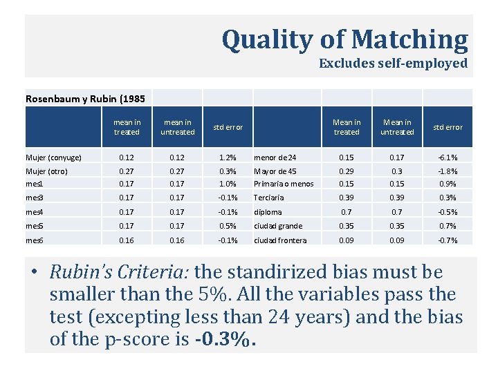
Quality of Matching Excludes self-employed Rosenbaum y Rubin (1985 mean in treated mean in untreated std error Mean in treated Mean in untreated std error Mujer (conyuge) 0. 12 1. 2% menor de 24 0. 15 0. 17 -6. 1% Mujer (otro) mes 1 0. 27 0. 17 0. 3% 1. 0% Mayor de 45 Primaria o menos 0. 29 0. 15 0. 3 0. 15 -1. 8% 0. 9% mes 3 0. 17 -0. 1% Terciaria 0. 39 0. 3% mes 4 0. 17 -0. 1% diploma 0. 7 -0. 5% mes 5 0. 17 0. 5% ciudad grande 0. 35 0. 7% mes 6 0. 16 -0. 1% ciudad frontera 0. 09 -0. 7% • Rubin’s Criteria: the standirized bias must be smaller than the 5%. All the variables pass the test (excepting less than 24 years) and the bias of the p-score is -0. 3%.

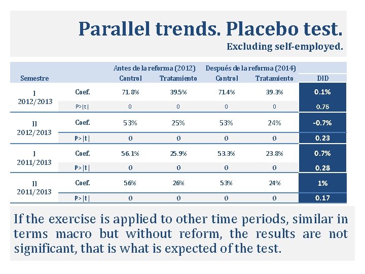
Parallel trends. Placebo test. Excluding self-employed. Antes de la reforma (2012) Control Tratamiento Semestre Después de la reforma (2014) Control Tratamiento DID I 2012/2013 Coef. 71. 8% 39. 5% 71. 4% 39. 3% 0. 1% P>|t| 0 0 0. 76 II 2012/2013 Coef. 53% 25% 53% 24% -0. 7% P>|t| 0 0 0. 23 Coef. 56. 1% 25. 9% 53. 3% 23. 8% 0. 7% P>|t| 0 0 0. 28 Coef. 56% 26% 53% 24% 1% P>|t| 0 0 0. 17 I 2011/2013 If the exercise is applied to other time periods, similar in terms macro but without reform, the results are not significant, that is what is expected of the test.

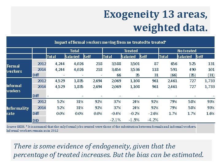
Exogeneity of the treatment. • This problem is one of the inconvenients of using MDID, and specially if cross section data is used. Van den Berg (2003), Blundell (2009) and Lechner (2011). • In this case, the workers may start earning more than a minimum wage to be benefited from the reform. – There is some evidence of endogeneity, given that the percentage of treated increases. But the bias can be estimated. • The effect is produced exclusively among individuals who earn less than a minimum wage. Whatsoever, making this individuals earn at least the minimum wage was the idea behind the reform.

Exogeneity 13 areas, weighted data. Impact of formal workers moving from no treated to treated* Total Salaried Total Formal workers Informal workers (e, thousands) 2012 2014 Diff 2012 2014 Informality Diff rate DID Self Total Treated Salaried Self No treated Salaried Self Total 4, 244 4, 529 4, 026 1, 835 218 2, 694 3, 588 3, 654 66 2, 069 3, 501 3, 536 35 1, 108 87 118 31 961 656 591 (66) 2, 461 525 490 (35) 727 131 101 (31) 1, 733 52% 0. 0% 31% 0. 0% 92% 0. 0% 37% -0. 4% 24% -0. 2% 92% -2. 6% 79% 1. 7% 58% 1. 7% 93% 1. 6% -2. 1% -1. 9% -4. 2% Source GEIH. * It is assumed that the only formal jobs created were those of the substitution between formals and informal workers. Informal workers remain as in 2012 There is some evidence of endogeneity, given that the percentage of treated increases. But the bias can be estimated.

Distribution effects.

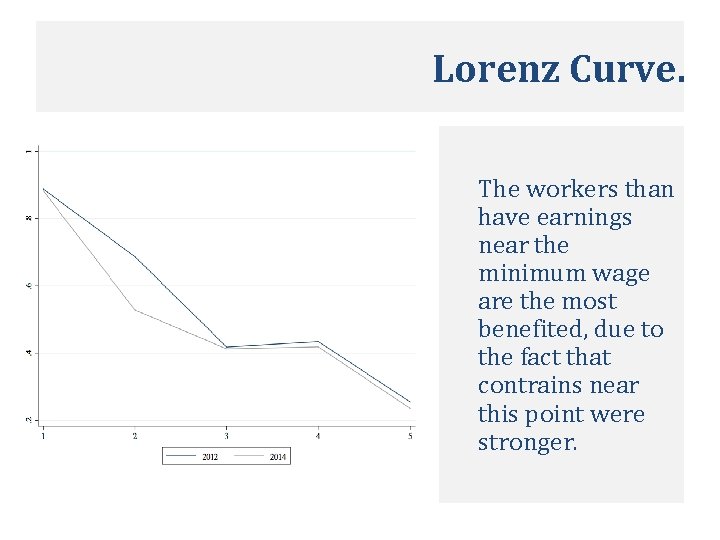
Lorenz Curve. The workers than have earnings near the minimum wage are the most benefited, due to the fact that contrains near this point were stronger.

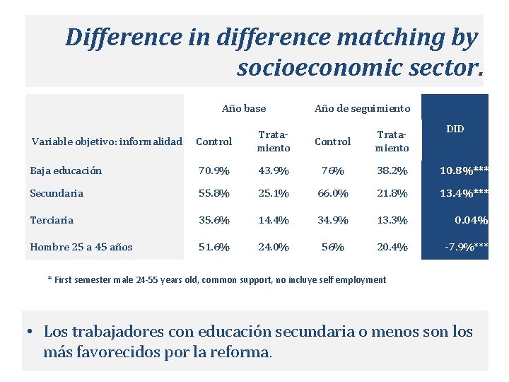
Difference in difference matching by socioeconomic sector. Año base Año de seguimiento Control Tratamiento DID Variable objetivo: informalidad Control Tratamiento Baja educación 70. 9% 43. 9% 76% 38. 2% 10. 8%*** Secundaria 55. 8% 25. 1% 66. 0% 21. 8% 13. 4%*** Terciaria 35. 6% 14. 4% 34. 9% 13. 3% 0. 04% Hombre 25 a 45 años 51. 6% 24. 0% 56% 20. 4% -7. 9%*** * First semester male 24 -55 years old, common support, no incluye self employment • Los trabajadores con educación secundaria o menos son los más favorecidos por la reforma.

The reduction of more than 10 points in payroll taxes reduced approximately 4 points in the informality rate in Colombia, of which approximately 2 points were due to formal workers that start wining more than a minimum wage and therefore were formalized.

Fin.