CPSC 533 Reinforcement Learning Paul Melenchuk Eva Wong

CPSC 533 Reinforcement Learning Paul Melenchuk Eva Wong Winson Yuen Kenneth Wong

Outline • • • Introduction Passive Learning in an Known Environment Passive Learning in an Unknown Environment Active Learning in an Unknown Environment Exploration Learning an Action Value Function • Generalization in Reinforcement Learning • Genetic Algorithms and Evolutionary Programming • Conclusion • Glossary

Introduction In which we examine how an agent can learn from success and failure, reward and punishment.

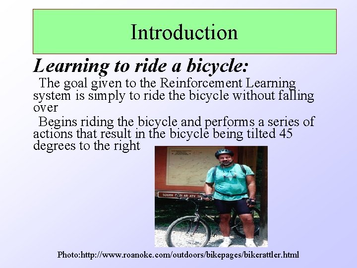
Introduction Learning to ride a bicycle: The goal given to the Reinforcement Learning system is simply to ride the bicycle without falling over Begins riding the bicycle and performs a series of actions that result in the bicycle being tilted 45 degrees to the right Photo: http: //www. roanoke. com/outdoors/bikepages/bikerattler. html

Introduction Learning to ride a bicycle: RL system turns the handle bars to the LEFT Result: CRASH!!! Receives negative reinforcement RL system turns the handle bars to the RIGHT Result: CRASH!!! Receives negative reinforcement

Introduction Learning to ride a bicycle: RL system has learned that the “state” of being titled 45 degrees to the right is bad Repeat trial using 40 degree to the right By performing enough of these trial-and-error interactions with the environment, the RL system will ultimately learn how to prevent the bicycle from ever falling over

Passive Learning in a Known Environment Passive Learner: A passive learner simply watches the world going by, and tries to learn the utility of being in various states. Another way to think of a passive learner is as an agent with a fixed policy trying to determine its benefits.

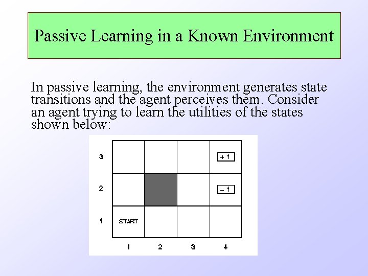
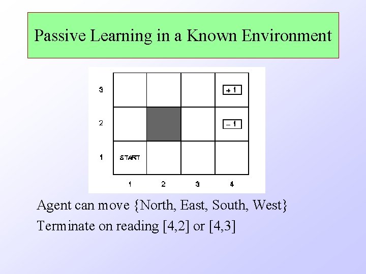
Passive Learning in a Known Environment In passive learning, the environment generates state transitions and the agent perceives them. Consider an agent trying to learn the utilities of the states shown below:

Passive Learning in a Known Environment Agent can move {North, East, South, West} Terminate on reading [4, 2] or [4, 3]

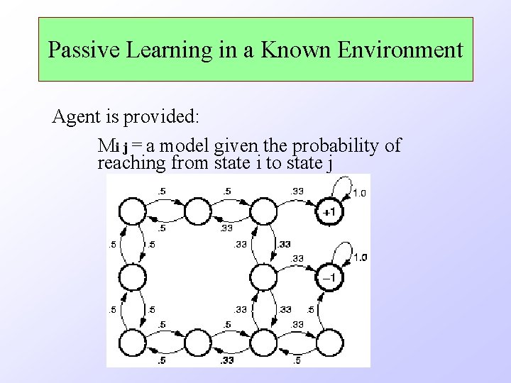
Passive Learning in a Known Environment Agent is provided: Mi j = a model given the probability of reaching from state i to state j

Passive Learning in a Known Environment the object is to use this information about rewards to learn the expected utility U(i) associated with each nonterminal state i Utilities can be learned using 3 approaches 1) LMS (least mean squares) 2) ADP (adaptive dynamic programming) 3) TD (temporal difference learning)

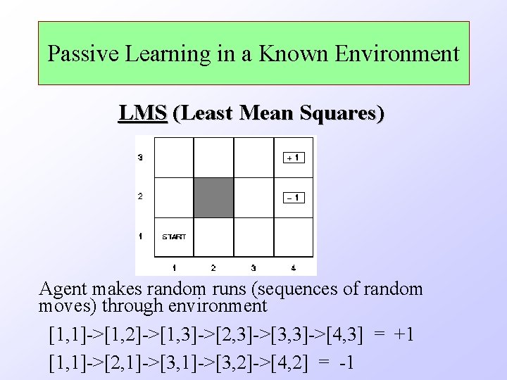
Passive Learning in a Known Environment LMS (Least Mean Squares) Agent makes random runs (sequences of random moves) through environment [1, 1]->[1, 2]->[1, 3]->[2, 3]->[3, 3]->[4, 3] = +1 [1, 1]->[2, 1]->[3, 2]->[4, 2] = -1

Passive Learning in a Known Environment LMS Collect statistics on final payoff for each state (eg. when on [2, 3], how often reached +1 vs -1 ? ) Learner computes average for each state Provably converges to true expected value (utilities) (Algorithm on page 602, Figure 20. 3)

Passive Learning in a Known Environment LMS Main Drawback: - slow convergence - it takes the agent well over a 1000 training sequences to get close to the correct value

Passive Learning in a Known Environment ADP (Adaptive Dynamic Programming) Uses the value or policy iteration algorithm to calculate exact utilities of states given an estimated model

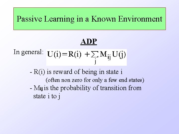
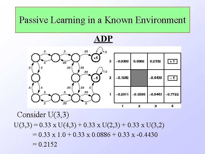
Passive Learning in a Known Environment ADP In general: - R(i) is reward of being in state i (often non zero for only a few end states) - Mij is the probability of transition from state i to j

Passive Learning in a Known Environment ADP Consider U(3, 3) = 0. 33 x U(4, 3) + 0. 33 x U(2, 3) + 0. 33 x U(3, 2) = 0. 33 x 1. 0 + 0. 33 x 0. 0886 + 0. 33 x -0. 4430 = 0. 2152

Passive Learning in a Known Environment ADP makes optimal use of the local constraints on utilities of states imposed by the neighborhood structure of the environment somewhat intractable for large state spaces

Passive Learning in a Known Environment TD (Temporal Difference Learning) The key is to use the observed transitions to adjust the values of the observed states so that they agree with the constraint equations

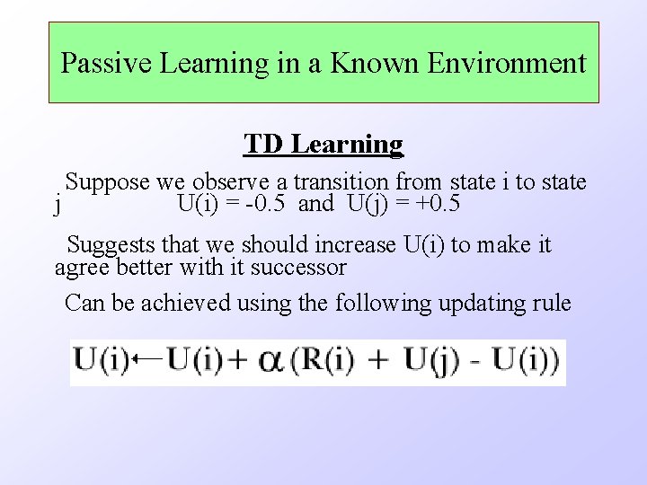
Passive Learning in a Known Environment TD Learning Suppose we observe a transition from state i to state j U(i) = -0. 5 and U(j) = +0. 5 Suggests that we should increase U(i) to make it agree better with it successor Can be achieved using the following updating rule

Passive Learning in a Known Environment TD Learning Performance: Runs “noisier” than LMS but smaller error Deal with observed states during sample runs (Not all instances, unlike ADP)

Passive Learning in an Unknown Environment Least Mean Square(LMS) approach and Temporal-Difference(TD) approach operate unchanged in an initially unknown environment. Adaptive Dynamic Programming(ADP) approach adds a step that updates an estimated model of the environment.

Passive Learning in an Unknown Environment ADP Approach • The environment model is learned by direct observation of transitions • The environment model M can be updated by keeping track of the percentage of times each state transitions to each of its neighbors

Passive Learning in an Unknown Environment ADP & TD Approaches • The ADP approach and the TD approach are closely related • Both try to make local adjustments to the utility estimates in order to make each state “agree” with its successors

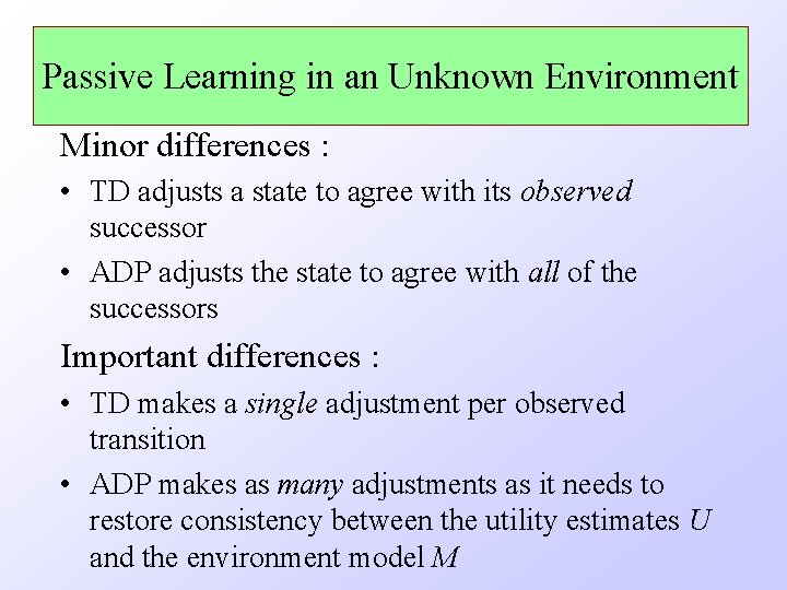
Passive Learning in an Unknown Environment Minor differences : • TD adjusts a state to agree with its observed successor • ADP adjusts the state to agree with all of the successors Important differences : • TD makes a single adjustment per observed transition • ADP makes as many adjustments as it needs to restore consistency between the utility estimates U and the environment model M

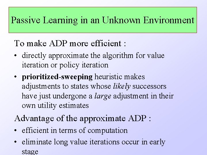
Passive Learning in an Unknown Environment To make ADP more efficient : • directly approximate the algorithm for value iteration or policy iteration • prioritized-sweeping heuristic makes adjustments to states whose likely successors have just undergone a large adjustment in their own utility estimates Advantage of the approximate ADP : • efficient in terms of computation • eliminate long value iterations occur in early stage

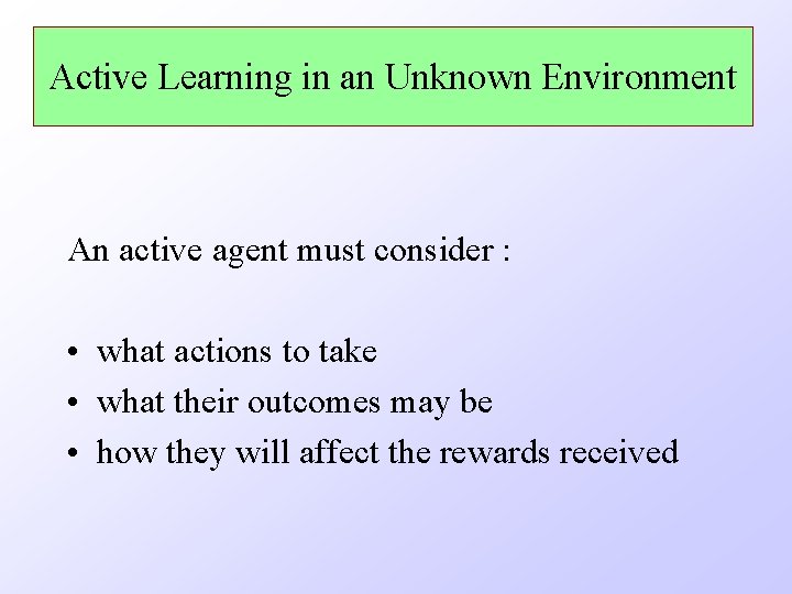
Active Learning in an Unknown Environment An active agent must consider : • what actions to take • what their outcomes may be • how they will affect the rewards received

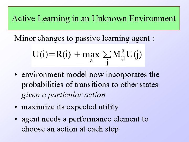
Active Learning in an Unknown Environment Minor changes to passive learning agent : • environment model now incorporates the probabilities of transitions to other states given a particular action • maximize its expected utility • agent needs a performance element to choose an action at each step

Active Learning in an Unknown Environment Active ADP Approach • need to learn the probability Maij of a transition instead of Mij • the input to the function will include the action taken

Active Learning in an Unknown Environment Active TD Approach • the model acquisition problem for the TD agent is identical to that for the ADP agent • the update rule remains unchanged • the TD algorithm will converge to the same values as ADP as the number of training sequences tends to infinity

Exploration Learning also involves the exploration of unknown areas Photo: http: //www. duke. edu/~icheese/cgeorge. html

Exploration An agent can benefit from actions in 2 ways immediate rewards received percepts

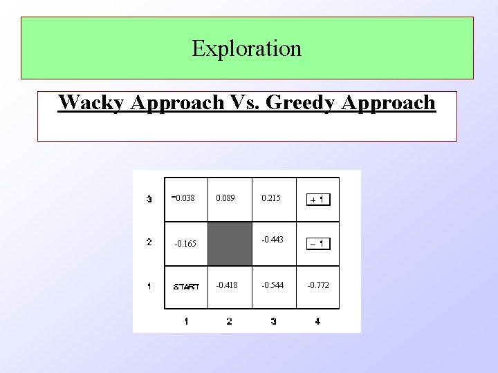
Exploration Wacky Approach Vs. Greedy Approach -0. 038 0. 089 0. 215 -0. 443 -0. 165 -0. 418 -0. 544 -0. 772

Exploration The Bandit Problem Photos: www. freetravel. net

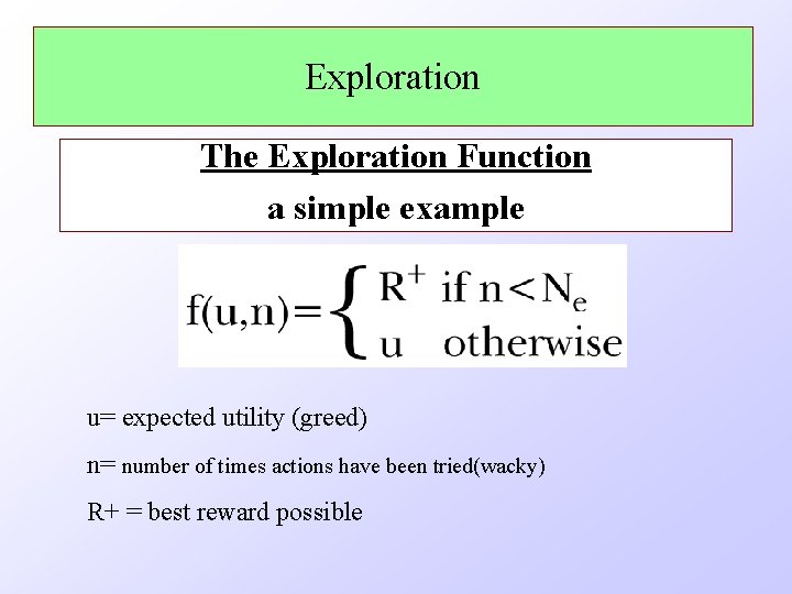
Exploration The Exploration Function a simple example u= expected utility (greed) n= number of times actions have been tried(wacky) R+ = best reward possible

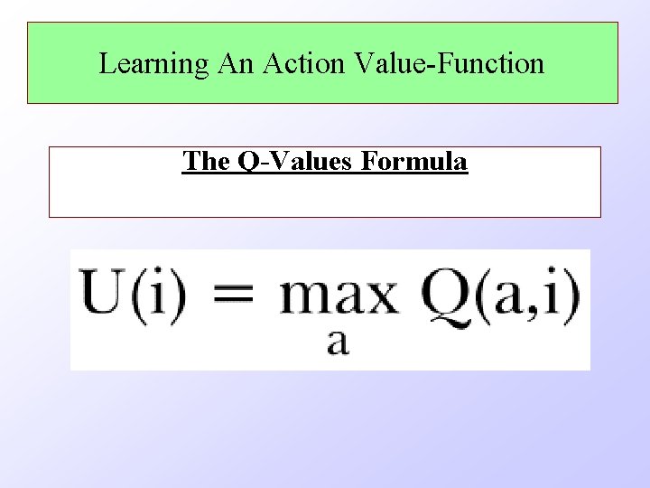
Learning An Action Value-Function What Are Q-Values?

Learning An Action Value-Function The Q-Values Formula

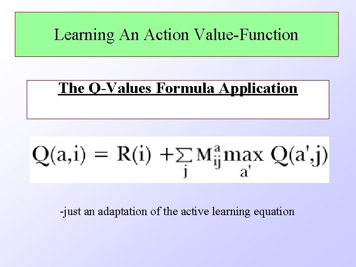
Learning An Action Value-Function The Q-Values Formula Application -just an adaptation of the active learning equation

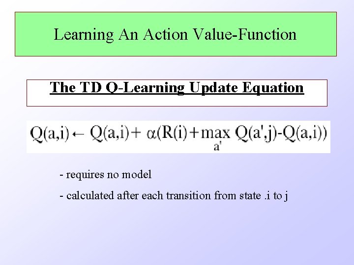
Learning An Action Value-Function The TD Q-Learning Update Equation - requires no model - calculated after each transition from state. i to j

Learning An Action Value-Function The TD Q-Learning Update Equation in Practice The TD-Gammon System(Tesauro) Program: Neurogammon - attempted to learn from self-play and implicit representation

Generalization In Reinforcement Learning Explicit Representation • we have assumed that all the functions learned by the agents(U, M, R, Q) are represented in tabular form • explicit representation involves one output value for each input tuple.

Generalization In Reinforcement Learning Explicit Representation • good for small state spaces, but the time to convergence and the time per iteration increase rapidly as the space gets larger • it may be possible to handle 10, 000 states or more • this suffices for 2 -dimensional, maze-like environments

Generalization In Reinforcement Learning Explicit Representation • Problem: more realistic worlds are out of question • eg. Chess & backgammon are tiny subsets of the real world, yet their state spaces contain 120 50 on the order of 10 to 10 states. So it would be absurd to suppose that one must visit all these states in order to learn how to play the game.

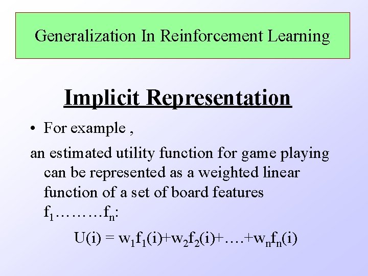
Generalization In Reinforcement Learning Implicit Representation • Overcome the explicit problem • a form that allows one to calculate the output for any input, but that is much more compact than the tabular form.

Generalization In Reinforcement Learning Implicit Representation • For example , an estimated utility function for game playing can be represented as a weighted linear function of a set of board features f 1………fn: U(i) = w 1 f 1(i)+w 2 f 2(i)+…. +wnfn(i)

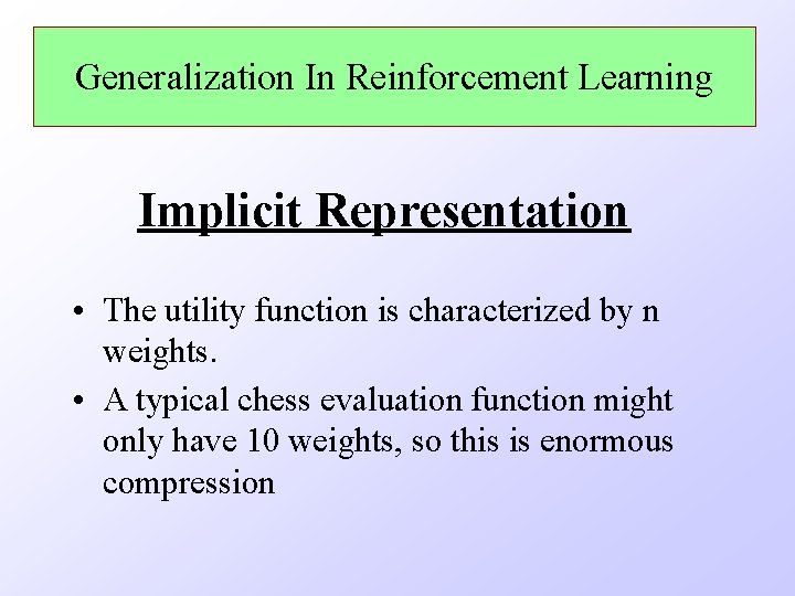
Generalization In Reinforcement Learning Implicit Representation • The utility function is characterized by n weights. • A typical chess evaluation function might only have 10 weights, so this is enormous compression

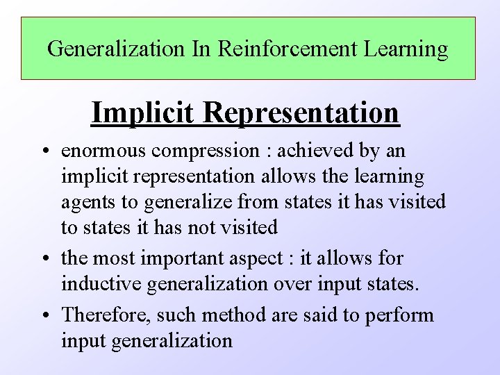
Generalization In Reinforcement Learning Implicit Representation • enormous compression : achieved by an implicit representation allows the learning agents to generalize from states it has visited to states it has not visited • the most important aspect : it allows for inductive generalization over input states. • Therefore, such method are said to perform input generalization

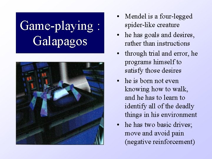
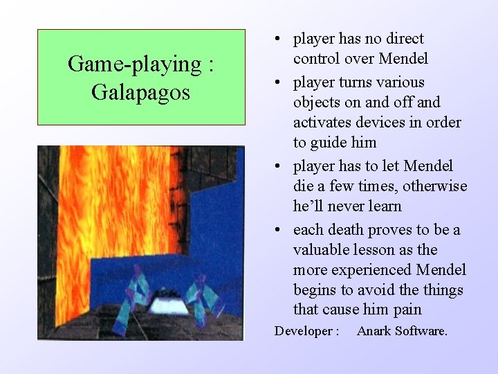
Game-playing : Galapagos • Mendel is a four-legged spider-like creature • he has goals and desires, rather than instructions • through trial and error, he programs himself to satisfy those desires • he is born not even knowing how to walk, and he has to learn to identify all of the deadly things in his environment • he has two basic drives; move and avoid pain (negative reinforcement)

Game-playing : Galapagos • player has no direct control over Mendel • player turns various objects on and off and activates devices in order to guide him • player has to let Mendel die a few times, otherwise he’ll never learn • each death proves to be a valuable lesson as the more experienced Mendel begins to avoid the things that cause him pain Developer : Anark Software.

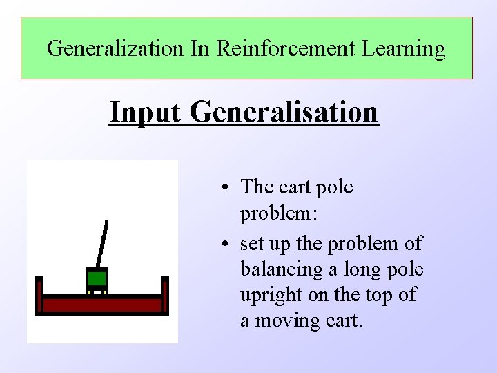
Generalization In Reinforcement Learning Input Generalisation • The cart pole problem: • set up the problem of balancing a long pole upright on the top of a moving cart.

Generalization In Reinforcement Learning Input Generalisation • The cart can be jerked left or right by a controller that observes x, x’, q, and q’ • the earliest work on learning for this problem was carried out by Michie and Chambers(1968) • their BOXES algorithm was able to balance the pole for over an hour after only about 30 trials.

Generalization In Reinforcement Learning Input Generalisation • The algorithm first discretized the 4 dimensional state into boxes, hence the name • it then ran trials until the pole fell over or the cart hit the end of the track. • Negative reinforcement was associated with the final action in the final box and then propagated back through the sequence

Generalization In Reinforcement Learning Input Generalisation • The discretization causes some problems when the apparatus was initialized in a different position • improvement : using the algorithm that adaptively partitions that state space according to the observed variation in the reward

Genetic Algorithms And Evolutionary Programming • Genetic algorithm starts with a set of one or more individuals that are successful, as measured by a fitness function • several choices for the individuals exist, such as: -Entire Agent function’s the fitness function is a performance measure or reward function - the analogy to natural selection is greatest

Genetic Algorithms And Evolutionary Programming • Genetic algorithm simply searches directly in the space of individuals, with the goal of finding one that maximizes the fitness function in a performance measure or reward function • search is parallel because each individual in the population can be seen as a separate search

Genetic Algorithms And Evolutionary Programming • component function of an agent • the fitness function is the critic or they can be anything at all that can be framed as an optimization problem • Evolutionary process: learn an agent function based on occasional rewards as supplied by the selection function, it can be seen as a form of reinforcement learning

Genetic Algorithms And Evolutionary Programming • Before we can apply Genetic algorithm to a problem, we need to answer 4 questions : 1. What is the fitness function? 2. How is an individual represented? 3. How are individuals selected? 4. How do individuals reproduce?

Genetic Algorithms And Evolutionary Programming What is fitness function? • Depends on the problem, but it is a function that takes an individual as input and returns a real number as output

Genetic Algorithms And Evolutionary Programming How is an individual represented? • In the classic genetic algorithm, an individual is represented as a string over a finite alphabet • each element of the string is called a gene • in genetic algorithm, we usually use the binary alphabet(1, 0) to represent DNA

Genetic Algorithms And Evolutionary Programming How are individuals selected ? • The selection strategy is usually randomized, with the probability of selection proportional to fitness • for example, if an individual X scores twice as high as Y on the fitness function, then X is twice as likely to be selected for reproduction than is Y. • selection is done with replacement

Genetic Algorithms And Evolutionary Programming How do individuals reproduce? • By cross-over and mutation • all the individuals that have been selected for reproduction are randomly paired • for each pair, a cross-over point is randomly chosen • cross-over point is a number in the range 1 to N

Genetic Algorithms And Evolutionary Programming How do individuals reproduce? • One offspring will get genes 1 through 10 from the first parent, and the rest from the second parent • the second offspring will get genes 1 through 10 from the second parent, and the rest from the first • however, each gene can be altered by random mutation to a different value

Conclusion • Passive Learning in a Known Environment • Passive Learning in an Unknown Environment • Active Learning in an Unknown Environment • Exploration • Learning an Action Value Function • Generalization in Reinforcement Learning • Genetic Algorithms and Evolutionary Programming

Resources And Glossary Information Source Russel, S. and P. Norvig (1995). Artificial Intelligence - A Modern Approach. Upper Saddle River, NJ, Prentice Hall Addition Information and Glossary of Keywords Available at http: //www. cpsc. ucalgary. ca/~paulme/533