Computer Aided Design and Manufacturing CADCAM Kartik Chandra

Computer Aided Design and Manufacturing (CAD/CAM) Kartik Chandra Bhagat Assistant Professor RTC INSTITUTE OF TECHNOLOGY, RANCHI JHARKHAND 1

Terminology CAD (Computer Aided Design): CAD is application of computers and graphics software to aid or enhance the product design from conceptualization to demonstration (The use of computer methods to develop the geometric model of the product in 3 -D form, such that the geometric and manufacturing requirements can be examined). CADD (Computer Aided Design and Drafting): Combining the CAD function with drafting to generate the production drawings of the parts for the purpose of the down stream processing. CAE (Computer Aided Engineering): the use of computer methods to support basic error checking analysis, optimization, manufacturing etc. of product design. 2

CAM (Computer Aided Manufacturing): Manufacturing Effective use of computer technology in manufacturing planning and control (The computer software used to develop the computer numerical control part programs). CIM (Computer Integrated Manufacturing): It is the phrase used to describe the complete automation of a manufacturing plant, with all processes functioning under computer control and digital information tying them together. CAP (Computer Aided Planning): Planning) The use of computer for many of the planning function such as material requirement planning, computer aided scheduling etc. CAPP: (Computer Aided Process Planning): The use of computer to generate the process plans for the complete manufacture of the product and parts. CATD (Computer Aided Tool Design): Computer assistance to be used for developing the tools for manufacture of products and parts. 3

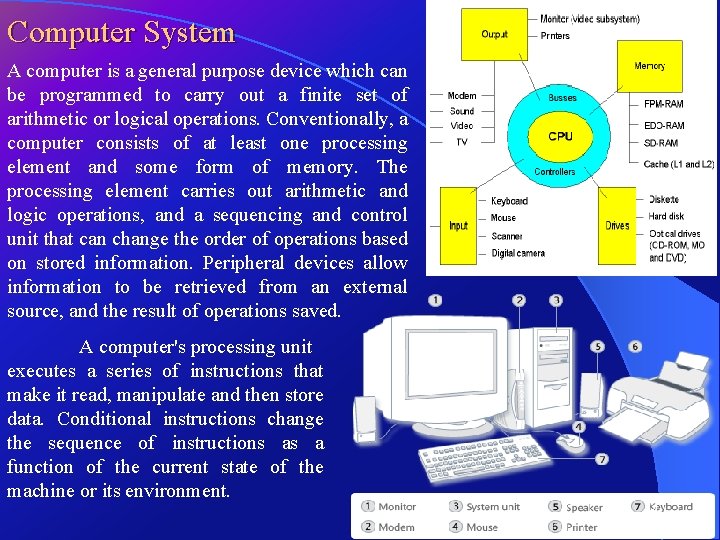
Computer System A computer is a general purpose device which can be programmed to carry out a finite set of arithmetic or logical operations. Conventionally, a computer consists of at least one processing element and some form of memory. The processing element carries out arithmetic and logic operations, and a sequencing and control unit that can change the order of operations based on stored information. Peripheral devices allow information to be retrieved from an external source, and the result of operations saved. A computer's processing unit executes a series of instructions that make it read, manipulate and then store data. Conditional instructions change the sequence of instructions as a function of the current state of the machine or its environment. 4

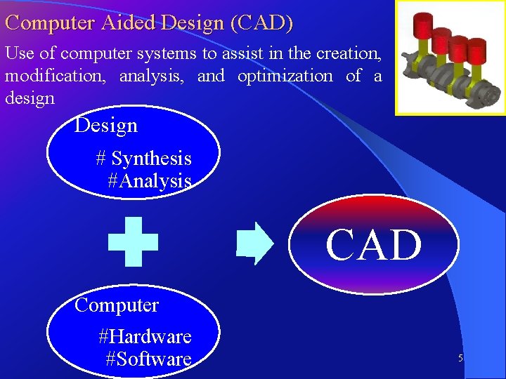
Computer Aided Design (CAD) Use of computer systems to assist in the creation, modification, analysis, and optimization of a design Design # Synthesis #Analysis CAD Computer #Hardware #Software 5

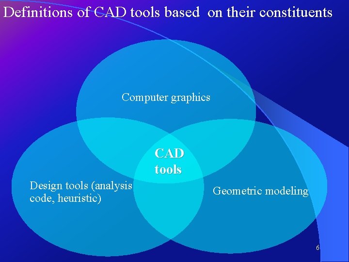
Definitions of CAD tools based on their constituents Computer graphics CAD tools Design tools (analysis code, heuristic) Geometric modeling 6

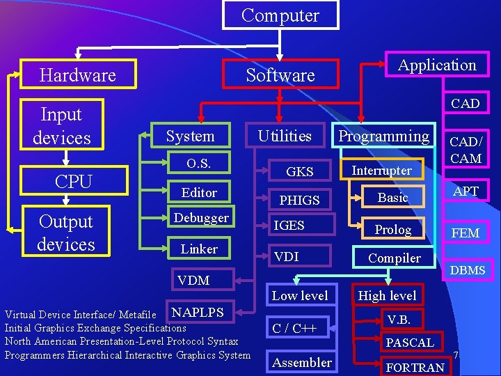
Computer Hardware Input devices CPU Output devices Software Application CAD System O. S. Editor Debugger Linker VDM Virtual Device Interface/ Metafile NAPLPS Initial Graphics Exchange Specifications North American Presentation-Level Protocol Syntax Programmers Hierarchical Interactive Graphics System Utilities GKS Programming Interrupter CAD/ CAM Basic APT IGES Prolog FEM VDI Compiler PHIGS Low level C / C++ Assembler DBMS High level V. B. PASCAL FORTRAN 7

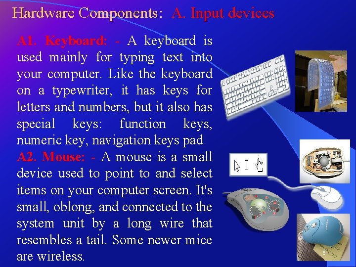
Hardware Components: A. Input devices A 1. Keyboard: - A keyboard is used mainly for typing text into your computer. Like the keyboard on a typewriter, it has keys for letters and numbers, but it also has special keys: function keys, numeric key, navigation keys pad A 2. Mouse: - A mouse is a small device used to point to and select items on your computer screen. It's small, oblong, and connected to the system unit by a long wire that resembles a tail. Some newer mice are wireless. 8

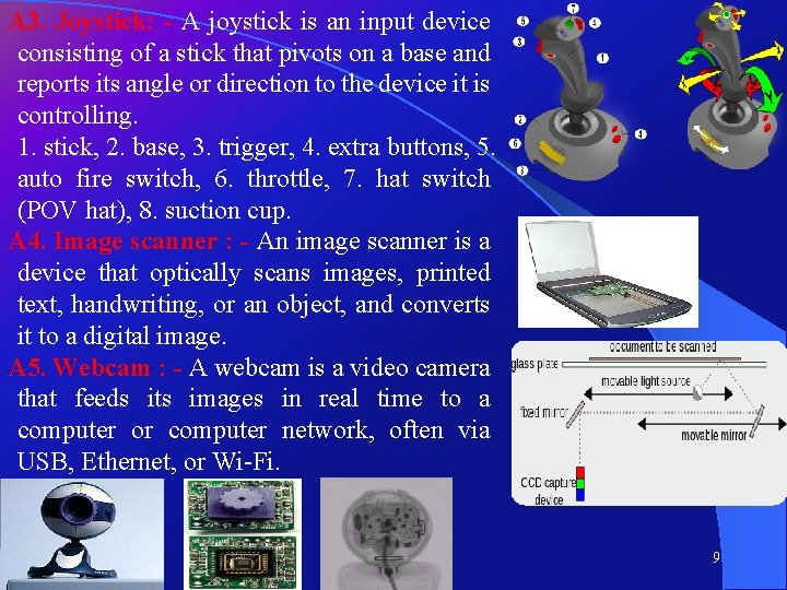
A 3. Joystick: - A joystick is an input device consisting of a stick that pivots on a base and reports its angle or direction to the device it is controlling. 1. stick, 2. base, 3. trigger, 4. extra buttons, 5. auto fire switch, 6. throttle, 7. hat switch (POV hat), 8. suction cup. A 4. Image scanner : - An image scanner is a device that optically scans images, printed text, handwriting, or an object, and converts it to a digital image. A 5. Webcam : - A webcam is a video camera that feeds its images in real time to a computer or computer network, often via USB, Ethernet, or Wi-Fi. 9

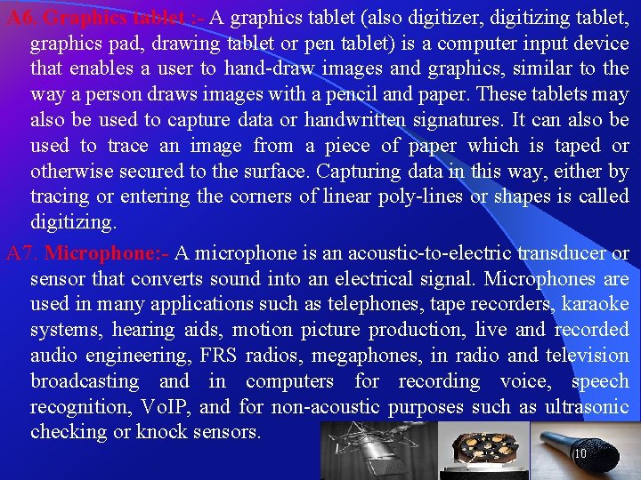
A 6. Graphics tablet : - A graphics tablet (also digitizer, digitizing tablet, graphics pad, drawing tablet or pen tablet) is a computer input device that enables a user to hand-draw images and graphics, similar to the way a person draws images with a pencil and paper. These tablets may also be used to capture data or handwritten signatures. It can also be used to trace an image from a piece of paper which is taped or otherwise secured to the surface. Capturing data in this way, either by tracing or entering the corners of linear poly-lines or shapes is called digitizing. A 7. Microphone: - A microphone is an acoustic-to-electric transducer or sensor that converts sound into an electrical signal. Microphones are used in many applications such as telephones, tape recorders, karaoke systems, hearing aids, motion picture production, live and recorded audio engineering, FRS radios, megaphones, in radio and television broadcasting and in computers for recording voice, speech recognition, Vo. IP, and for non-acoustic purposes such as ultrasonic checking or knock sensors. 10

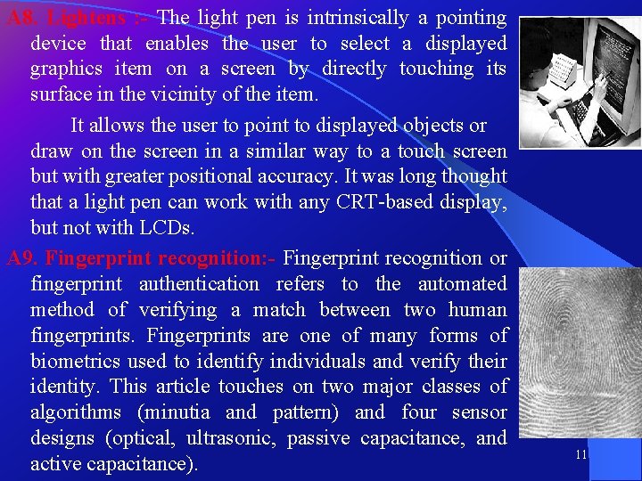
A 8. Lightens : - The light pen is intrinsically a pointing device that enables the user to select a displayed graphics item on a screen by directly touching its surface in the vicinity of the item. It allows the user to point to displayed objects or draw on the screen in a similar way to a touch screen but with greater positional accuracy. It was long thought that a light pen can work with any CRT-based display, but not with LCDs. A 9. Fingerprint recognition: - Fingerprint recognition or fingerprint authentication refers to the automated method of verifying a match between two human fingerprints. Fingerprints are one of many forms of biometrics used to identify individuals and verify their identity. This article touches on two major classes of algorithms (minutia and pattern) and four sensor designs (optical, ultrasonic, passive capacitance, and active capacitance). 11

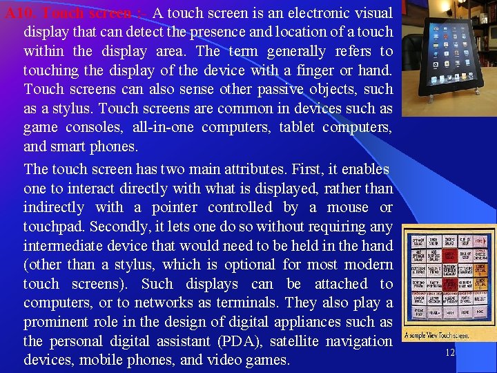
A 10. Touch screen : - A touch screen is an electronic visual display that can detect the presence and location of a touch within the display area. The term generally refers to touching the display of the device with a finger or hand. Touch screens can also sense other passive objects, such as a stylus. Touch screens are common in devices such as game consoles, all-in-one computers, tablet computers, and smart phones. The touch screen has two main attributes. First, it enables one to interact directly with what is displayed, rather than indirectly with a pointer controlled by a mouse or touchpad. Secondly, it lets one do so without requiring any intermediate device that would need to be held in the hand (other than a stylus, which is optional for most modern touch screens). Such displays can be attached to computers, or to networks as terminals. They also play a prominent role in the design of digital appliances such as the personal digital assistant (PDA), satellite navigation devices, mobile phones, and video games. 12

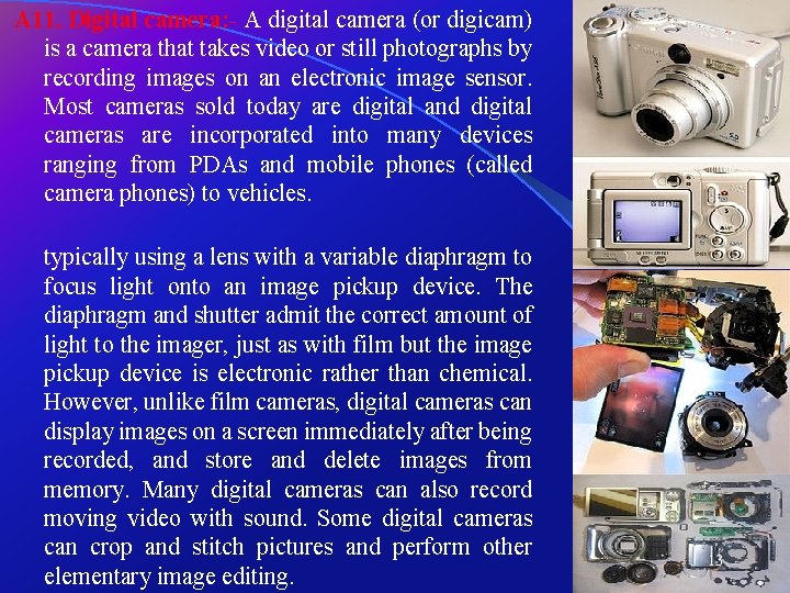
A 11. Digital camera: - A digital camera (or digicam) is a camera that takes video or still photographs by recording images on an electronic image sensor. Most cameras sold today are digital and digital cameras are incorporated into many devices ranging from PDAs and mobile phones (called camera phones) to vehicles. typically using a lens with a variable diaphragm to focus light onto an image pickup device. The diaphragm and shutter admit the correct amount of light to the imager, just as with film but the image pickup device is electronic rather than chemical. However, unlike film cameras, digital cameras can display images on a screen immediately after being recorded, and store and delete images from memory. Many digital cameras can also record moving video with sound. Some digital cameras can crop and stitch pictures and perform other elementary image editing. 13

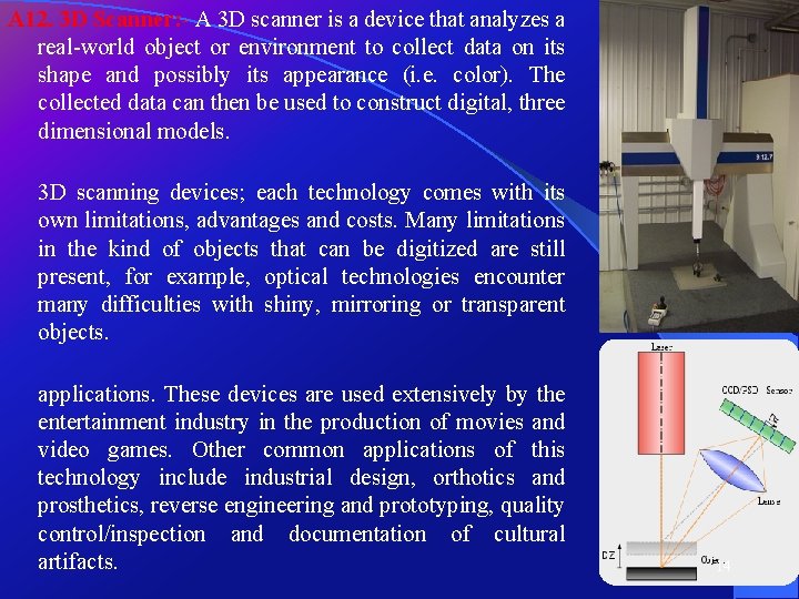
A 12. 3 D Scanner: - A 3 D scanner is a device that analyzes a real-world object or environment to collect data on its shape and possibly its appearance (i. e. color). The collected data can then be used to construct digital, three dimensional models. 3 D scanning devices; each technology comes with its own limitations, advantages and costs. Many limitations in the kind of objects that can be digitized are still present, for example, optical technologies encounter many difficulties with shiny, mirroring or transparent objects. applications. These devices are used extensively by the entertainment industry in the production of movies and video games. Other common applications of this technology include industrial design, orthotics and prosthetics, reverse engineering and prototyping, quality control/inspection and documentation of cultural artifacts. 14

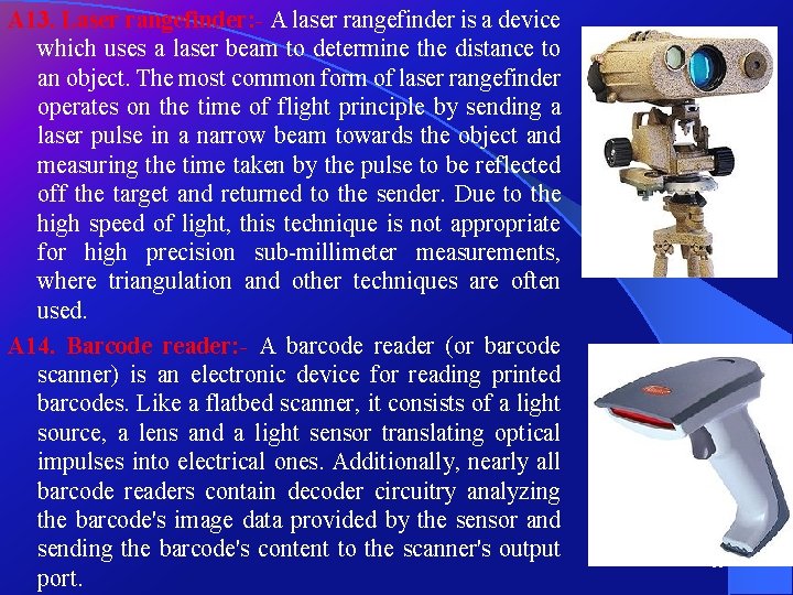
A 13. Laser rangefinder: - A laser rangefinder is a device which uses a laser beam to determine the distance to an object. The most common form of laser rangefinder operates on the time of flight principle by sending a laser pulse in a narrow beam towards the object and measuring the time taken by the pulse to be reflected off the target and returned to the sender. Due to the high speed of light, this technique is not appropriate for high precision sub-millimeter measurements, where triangulation and other techniques are often used. A 14. Barcode reader: - A barcode reader (or barcode scanner) is an electronic device for reading printed barcodes. Like a flatbed scanner, it consists of a light source, a lens and a light sensor translating optical impulses into electrical ones. Additionally, nearly all barcode readers contain decoder circuitry analyzing the barcode's image data provided by the sensor and sending the barcode's content to the scanner's output port. 15

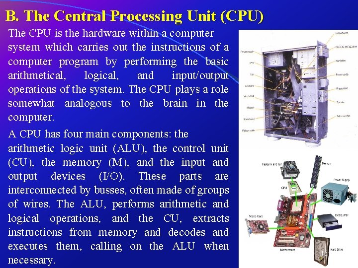
B. The Central Processing Unit (CPU) The CPU is the hardware within a computer system which carries out the instructions of a computer program by performing the basic arithmetical, logical, and input/output operations of the system. The CPU plays a role somewhat analogous to the brain in the computer. A CPU has four main components: the arithmetic logic unit (ALU), the control unit (CU), the memory (M), and the input and output devices (I/O). These parts are interconnected by busses, often made of groups of wires. The ALU, performs arithmetic and logical operations, and the CU, extracts instructions from memory and decodes and executes them, calling on the ALU when necessary. 16

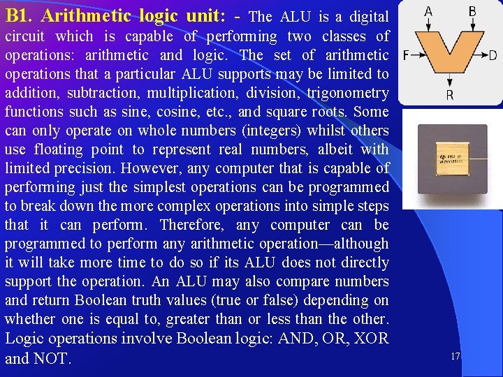
B 1. Arithmetic logic unit: - The ALU is a digital circuit which is capable of performing two classes of operations: arithmetic and logic. The set of arithmetic operations that a particular ALU supports may be limited to addition, subtraction, multiplication, division, trigonometry functions such as sine, cosine, etc. , and square roots. Some can only operate on whole numbers (integers) whilst others use floating point to represent real numbers, albeit with limited precision. However, any computer that is capable of performing just the simplest operations can be programmed to break down the more complex operations into simple steps that it can perform. Therefore, any computer can be programmed to perform any arithmetic operation—although it will take more time to do so if its ALU does not directly support the operation. An ALU may also compare numbers and return Boolean truth values (true or false) depending on whether one is equal to, greater than or less than the other. Logic operations involve Boolean logic: AND, OR, XOR and NOT. 17

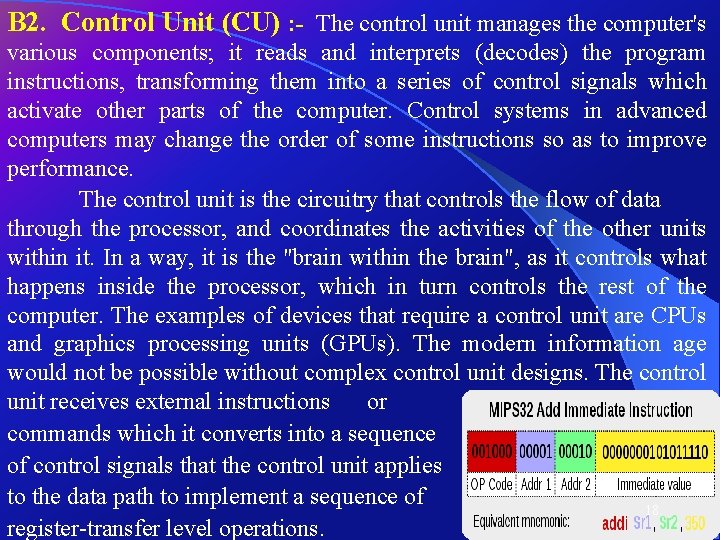
B 2. Control Unit (CU) : - The control unit manages the computer's various components; it reads and interprets (decodes) the program instructions, transforming them into a series of control signals which activate other parts of the computer. Control systems in advanced computers may change the order of some instructions so as to improve performance. The control unit is the circuitry that controls the flow of data through the processor, and coordinates the activities of the other units within it. In a way, it is the "brain within the brain", as it controls what happens inside the processor, which in turn controls the rest of the computer. The examples of devices that require a control unit are CPUs and graphics processing units (GPUs). The modern information age would not be possible without complex control unit designs. The control unit receives external instructions or commands which it converts into a sequence of control signals that the control unit applies to the data path to implement a sequence of 18 register-transfer level operations.

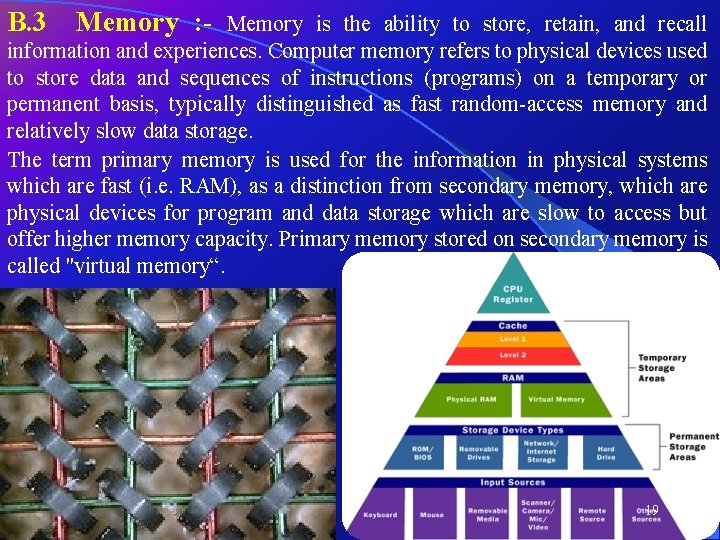
B. 3 Memory : - Memory is the ability to store, retain, and recall information and experiences. Computer memory refers to physical devices used to store data and sequences of instructions (programs) on a temporary or permanent basis, typically distinguished as fast random-access memory and relatively slow data storage. The term primary memory is used for the information in physical systems which are fast (i. e. RAM), as a distinction from secondary memory, which are physical devices for program and data storage which are slow to access but offer higher memory capacity. Primary memory stored on secondary memory is called "virtual memory“. 19

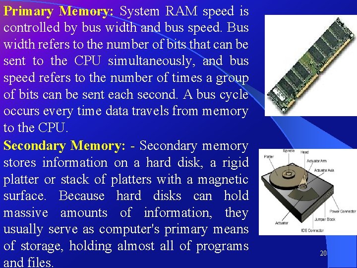
Primary Memory: System RAM speed is controlled by bus width and bus speed. Bus width refers to the number of bits that can be sent to the CPU simultaneously, and bus speed refers to the number of times a group of bits can be sent each second. A bus cycle occurs every time data travels from memory to the CPU. Secondary Memory: - Secondary memory stores information on a hard disk, a rigid platter or stack of platters with a magnetic surface. Because hard disks can hold massive amounts of information, they usually serve as computer's primary means of storage, holding almost all of programs and files. 20

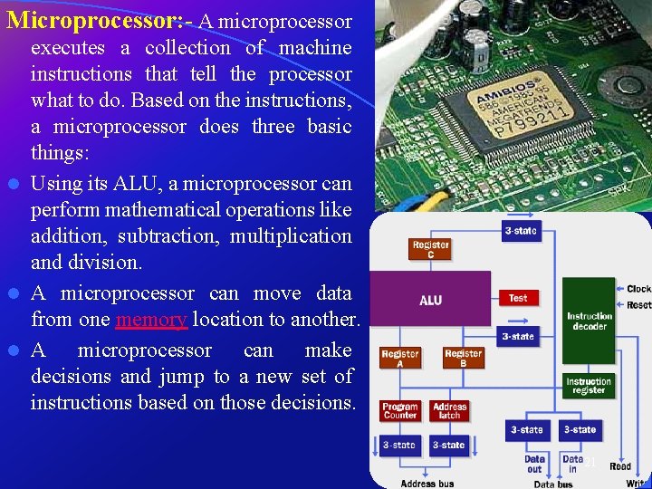
Microprocessor: - A microprocessor executes a collection of machine instructions that tell the processor what to do. Based on the instructions, a microprocessor does three basic things: l Using its ALU, a microprocessor can perform mathematical operations like addition, subtraction, multiplication and division. l A microprocessor can move data from one memory location to another. l A microprocessor can make decisions and jump to a new set of instructions based on those decisions. 21

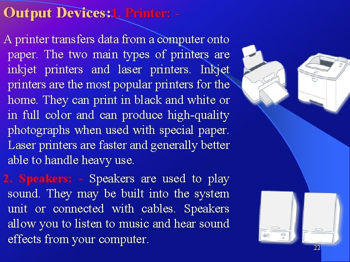
Output Devices: 1. Printer: A printer transfers data from a computer onto paper. The two main types of printers are inkjet printers and laser printers. Inkjet printers are the most popular printers for the home. They can print in black and white or in full color and can produce high-quality photographs when used with special paper. Laser printers are faster and generally better able to handle heavy use. 2. Speakers: - Speakers are used to play sound. They may be built into the system unit or connected with cables. Speakers allow you to listen to music and hear sound effects from your computer. 22

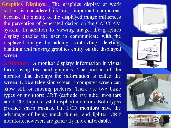
Graphics Displays: - The graphics display of work station is considered its most important component because the quality of the displayed image influences the perception of generated design on the CAD/CAM system. In addition to viewing image, the graphics display enables the user to communicate with the displayed image by adding, subtracting, deleting, blanking and moving graphics entity on the displayed screen. 3. Monitor: - A monitor displays information in visual form, using text and graphics. The portion of the monitor that displays the information is called the screen. Like a television screen, a computer screen can show still or moving pictures. There are two basic types of monitors: CRT (cathode ray tube) monitors and LCD (liquid crystal display) monitors. Both types produce sharp images, but LCD monitors have the advantage of being much thinner and lighter. CRT monitors, however, are generally more affordable. 23

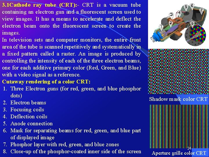
3. 1 Cathode ray tube (CRT): - CRT is a vacuum tube containing an electron gun and a fluorescent screen used to view images. It has a means to accelerate and deflect the electron beam onto the fluorescent screen to create the images. In television sets and computer monitors, the entire front area of the tube is scanned repetitively and systematically in a fixed pattern called a raster. An image is produced by controlling the intensity of each of the three electron beams, one for each additive primary color (Red, Green, and Blue) with a video signal as a reference. Cutaway rendering of a color CRT: 1. Three Electron guns (for red, green, and blue phosphor dots) 2. Electron beams 3. Focusing coils 4. Deflection coils 5. Anode connection 6. Mask for separating beams for red, green, and blue part of displayed image 7. Phosphor layer with red, green, and blue zones 8. Close-up of the phosphor-coated inner side of the screen Shadow mask color CRT 24 Aperture grille color CRT

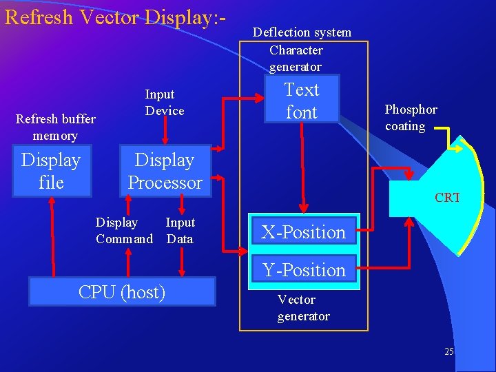
Refresh Vector Display: - Refresh buffer memory Display file Input Device Deflection system Character generator Text font Display Processor Display Input Command Data Phosphor coating CRT X-Position Y-Position CPU (host) Vector generator 25

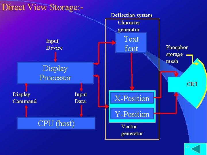
Direct View Storage: - Deflection system Character generator Text font Input Device Display Processor Display Command Phosphor storage mesh CRT Input Data X-Position Y-Position CPU (host) Vector generator 26

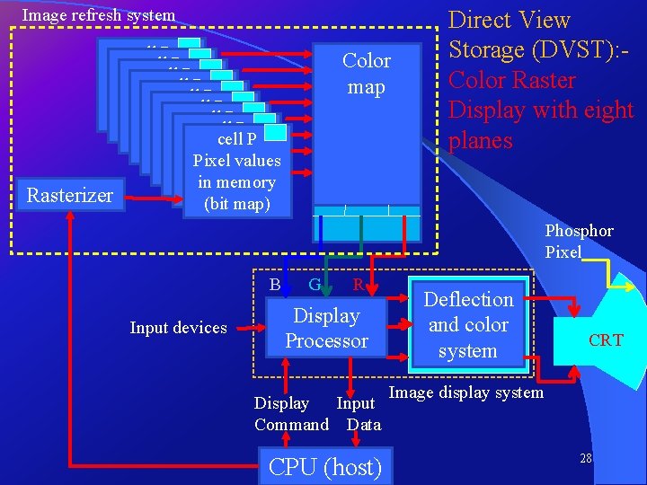
Image refresh system cell P Pixel values cell P in Pixel memory values cell P (bit inmap) memory Pixel values cell P (bit inmap) memory Pixel values (bit inmap) memory (bit map) Rasterizer (bit map) Color map Direct View Storage (DVST): Color Raster Display with eight planes Phosphor Pixel B Input devices G R Display Processor Display Input Command Data CPU (host) Deflection and color system CRT Image display system 27

Image refresh system cell P Pixel values cell P in Pixel memory values cell P (bit inmap) memory Pixel values cell P (bit inmap) memory Pixel values (bit inmap) memory (bit map) Rasterizer (bit map) Color map Direct View Storage (DVST): Color Raster Display with eight planes Phosphor Pixel B Input devices G R Display Processor Display Input Command Data CPU (host) Deflection and color system CRT Image display system 28

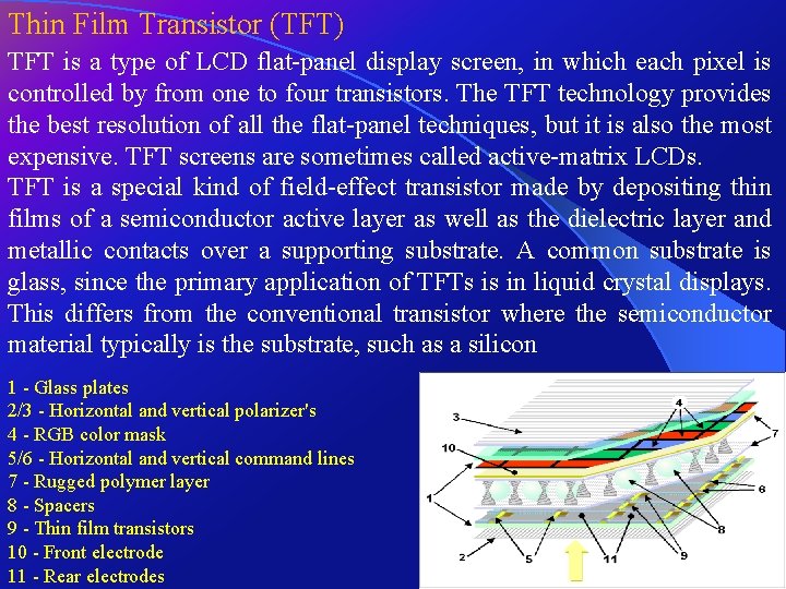
Thin Film Transistor (TFT) TFT is a type of LCD flat-panel display screen, in which each pixel is controlled by from one to four transistors. The TFT technology provides the best resolution of all the flat-panel techniques, but it is also the most expensive. TFT screens are sometimes called active-matrix LCDs. TFT is a special kind of field-effect transistor made by depositing thin films of a semiconductor active layer as well as the dielectric layer and metallic contacts over a supporting substrate. A common substrate is glass, since the primary application of TFTs is in liquid crystal displays. This differs from the conventional transistor where the semiconductor material typically is the substrate, such as a silicon 1 - Glass plates 2/3 - Horizontal and vertical polarizer's 4 - RGB color mask 5/6 - Horizontal and vertical command lines 7 - Rugged polymer layer 8 - Spacers 9 - Thin film transistors 10 - Front electrode 11 - Rear electrodes 29

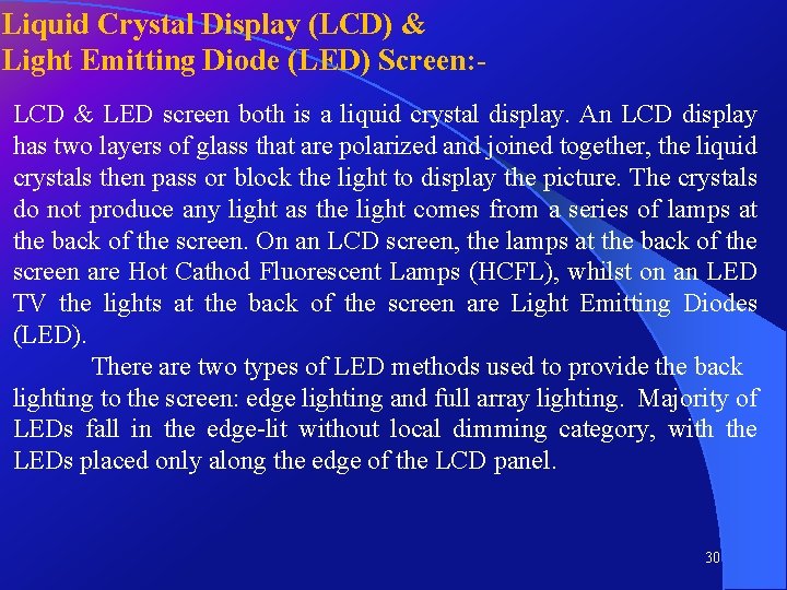
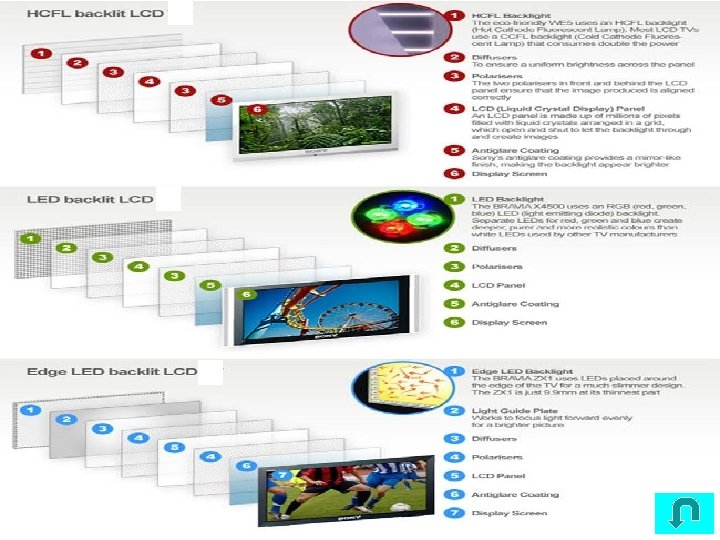
Liquid Crystal Display (LCD) & Light Emitting Diode (LED) Screen: LCD & LED screen both is a liquid crystal display. An LCD display has two layers of glass that are polarized and joined together, the liquid crystals then pass or block the light to display the picture. The crystals do not produce any light as the light comes from a series of lamps at the back of the screen. On an LCD screen, the lamps at the back of the screen are Hot Cathod Fluorescent Lamps (HCFL), whilst on an LED TV the lights at the back of the screen are Light Emitting Diodes (LED). There are two types of LED methods used to provide the back lighting to the screen: edge lighting and full array lighting. Majority of LEDs fall in the edge-lit without local dimming category, with the LEDs placed only along the edge of the LCD panel. 30

31

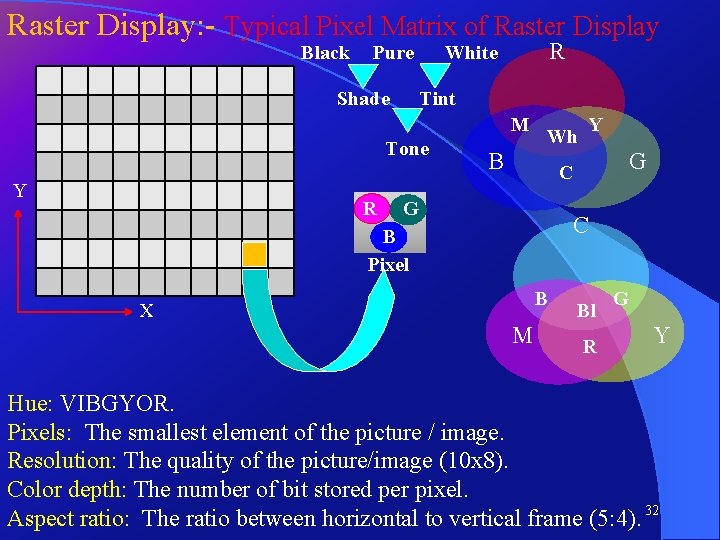
Raster Display: - Typical Pixel Matrix of Raster Display Black Pure Shade R White Tint M Tone Y R Wh B Y G C B Pixel B X M Bl R G Y Hue: VIBGYOR. Pixels: The smallest element of the picture / image. Resolution: The quality of the picture/image (10 x 8). Color depth: The number of bit stored per pixel. Aspect ratio: The ratio between horizontal to vertical frame (5: 4). 32

Resolution: - The resolution are the number of pixel presents along the entire length and width of an image/ picture. The size of the image/ picture is known as frame. The resolution are two distinctly different terms image resolution and screen resolution. Image resolution refers to the pixel spacing of an image/picture i. e. the distance from one pixel to next pixel. It is measured by PPI. The screen resolution is refer to the internal surface of the monitor screen which is coated with RGB phosphor material that glows when struck by a stream of electron. The coated material is arranged into an array of million of tiny cells RGB usually called dots. The dots pitch is the distance between adjacent sets of RGB dots. It is measured by DPI: the shortest distance between any two dots of same color. Refresh rate: - The screen image is "refreshed" many times per second. Refresh rates are measured in Hertz (HZ), which means "times per second". Video RAM: - All video cards have some RAM. How much depends on the desired colour depth. Video cards usually have 1, 2 or 4 MB RAM 33 for normal usage.

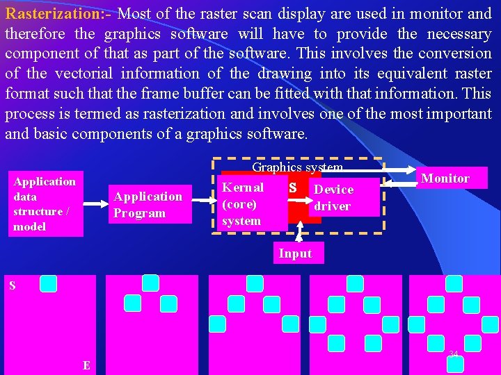
Rasterization: - Most of the raster scan display are used in monitor and therefore the graphics software will have to provide the necessary component of that as part of the software. This involves the conversion of the vectorial information of the drawing into its equivalent raster format such that the frame buffer can be fitted with that information. This process is termed as rasterization and involves one of the most important and basic components of a graphics software. Application data structure / model Application Program Graphics system Kernal Graphics Device (core) driver system Monitor Input S E 34

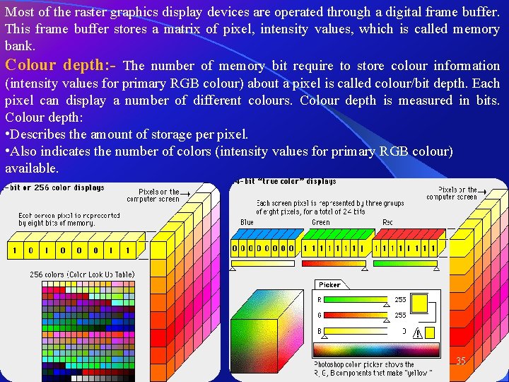
Most of the raster graphics display devices are operated through a digital frame buffer. This frame buffer stores a matrix of pixel, intensity values, which is called memory bank. Colour depth: - The number of memory bit require to store colour information (intensity values for primary RGB colour) about a pixel is called colour/bit depth. Each pixel can display a number of different colours. Colour depth is measured in bits. Colour depth: • Describes the amount of storage per pixel. • Also indicates the number of colors (intensity values for primary RGB colour) available. 35

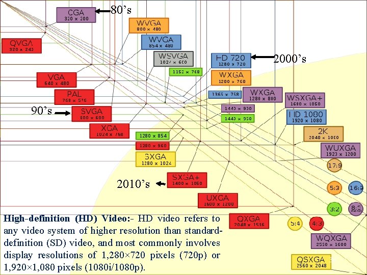
80’s 2000’s 90’s 2010’s High-definition (HD) Video: - HD video refers to any video system of higher resolution than standarddefinition (SD) video, and most commonly involves display resolutions of 1, 280× 720 pixels (720 p) or 1, 920× 1, 080 pixels (1080 i/1080 p). 36

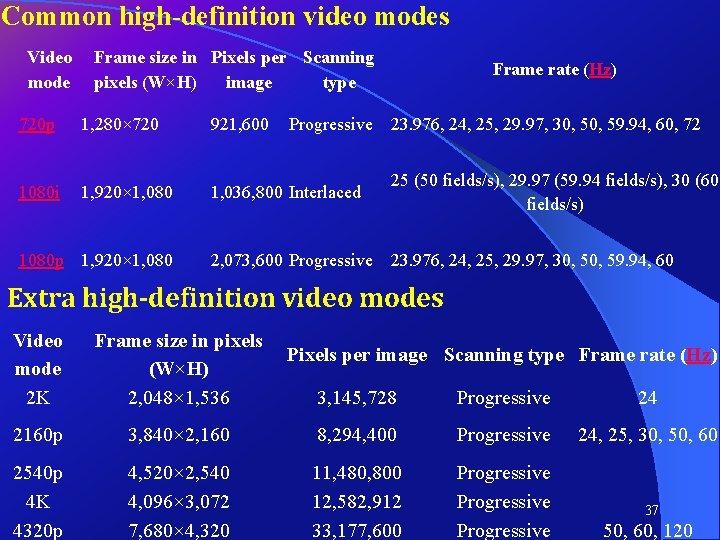
Common high-definition video modes Video mode Frame size in Pixels per Scanning pixels (W×H) image type 720 p 1, 280× 720 921, 600 1080 i 1, 920× 1, 080 1, 036, 800 Interlaced 25 (50 fields/s), 29. 97 (59. 94 fields/s), 30 (60 fields/s) 2, 073, 600 Progressive 23. 976, 24, 25, 29. 97, 30, 59. 94, 60 1080 p 1, 920× 1, 080 Progressive Frame rate (Hz) 23. 976, 24, 25, 29. 97, 30, 59. 94, 60, 72 Extra high-definition video modes Video mode 2 K Frame size in pixels (W×H) 2, 048× 1, 536 2160 p 2540 p 4 K 4320 p Pixels per image Scanning type Frame rate (Hz) 3, 145, 728 Progressive 24 3, 840× 2, 160 8, 294, 400 Progressive 24, 25, 30, 50, 60 4, 520× 2, 540 4, 096× 3, 072 7, 680× 4, 320 11, 480, 800 12, 582, 912 33, 177, 600 Progressive 37 50, 60, 120

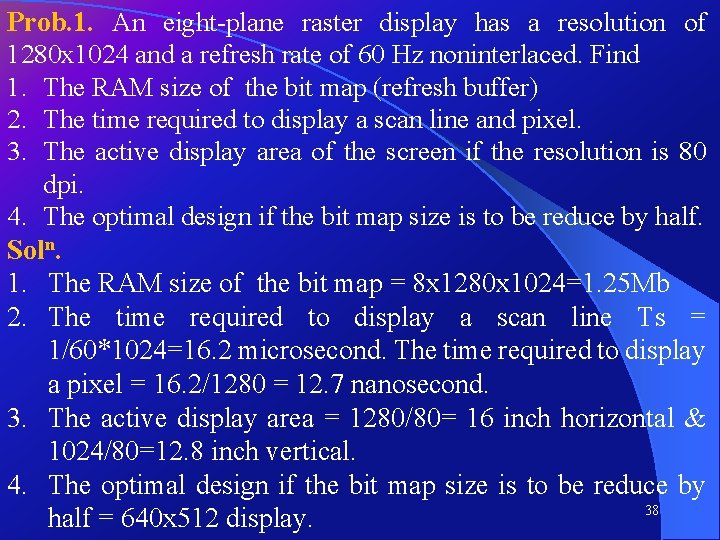
Prob. 1. An eight-plane raster display has a resolution of 1280 x 1024 and a refresh rate of 60 Hz noninterlaced. Find 1. The RAM size of the bit map (refresh buffer) 2. The time required to display a scan line and pixel. 3. The active display area of the screen if the resolution is 80 dpi. 4. The optimal design if the bit map size is to be reduce by half. Soln. 1. The RAM size of the bit map = 8 x 1280 x 1024=1. 25 Mb 2. The time required to display a scan line Ts = 1/60*1024=16. 2 microsecond. The time required to display a pixel = 16. 2/1280 = 12. 7 nanosecond. 3. The active display area = 1280/80= 16 inch horizontal & 1024/80=12. 8 inch vertical. 4. The optimal design if the bit map size is to be reduce by 38 half = 640 x 512 display.

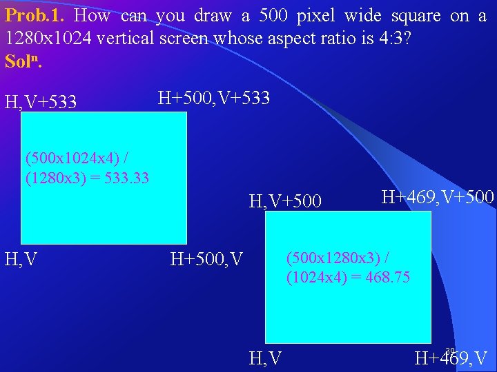
Prob. 1. How can you draw a 500 pixel wide square on a 1280 x 1024 vertical screen whose aspect ratio is 4: 3? Soln. H, V+533 H+500, V+533 (500 x 1024 x 4) / (1280 x 3) = 533. 33 H, V+500 H, V H+500, V H+469, V+500 (500 x 1280 x 3) / (1024 x 4) = 468. 75 H, V 39 H+469, V

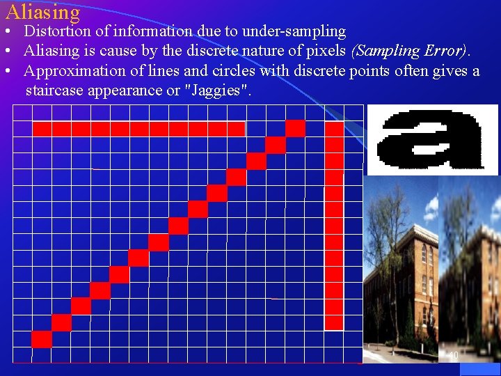
Aliasing • Distortion of information due to under-sampling • Aliasing is cause by the discrete nature of pixels (Sampling Error). • Approximation of lines and circles with discrete points often gives a staircase appearance or "Jaggies". 40

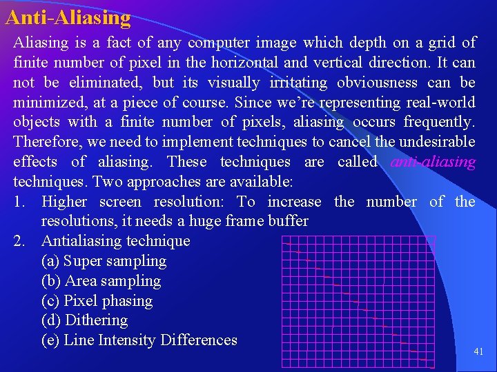
Anti-Aliasing is a fact of any computer image which depth on a grid of finite number of pixel in the horizontal and vertical direction. It can not be eliminated, but its visually irritating obviousness can be minimized, at a piece of course. Since we’re representing real-world objects with a finite number of pixels, aliasing occurs frequently. Therefore, we need to implement techniques to cancel the undesirable effects of aliasing. These techniques are called anti-aliasing techniques. Two approaches are available: 1. Higher screen resolution: To increase the number of the resolutions, it needs a huge frame buffer 2. Antialiasing technique (a) Super sampling (b) Area sampling (c) Pixel phasing (d) Dithering (e) Line Intensity Differences 41

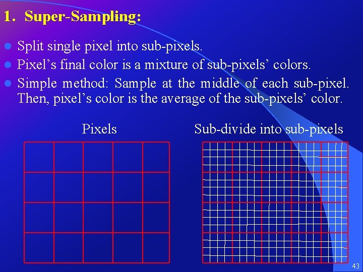
Anti-aliasing Techniques: Vary pixel intensities along boundaries to smooth the edge. 1. Super sampling: Compute intensities at sub-pixel grid positions and combine the results to obtain the pixel intensity. 2. Area sampling 2. 1 Unweighted area sampling: a). Find pixel intensity by calculating the areas of overlap of each pixel within the objects to be displayed. b). Pixel intensity is proportional to the amount of area covered. 2. 2 Weighted area sampling: Define a weighting function that determines the influence on the intensity of the pixel. 3. Pixel phasing: Lines are smoothed by moving the electron beam to a closer approximate of the mathematical line. Pixel positions can be shifted by a fraction of a pixel diameter (1/4, 1/2, or 3/4) to plot points closer to the mathematical line. 4. Dithering: Combining pixel of available colour 5. Line Intensity Differences: The diagonal line appears less bright than the horizontal. (The diagonal line is longer than the horizontal line by a factor of sqrt(2)). Total intensity is proportional to their length. 42

1. Super-Sampling: Split single pixel into sub-pixels. l Pixel’s final color is a mixture of sub-pixels’ colors. l Simple method: Sample at the middle of each sub-pixel. Then, pixel’s color is the average of the sub-pixels’ color. l Pixels Sub-divide into sub-pixels 43

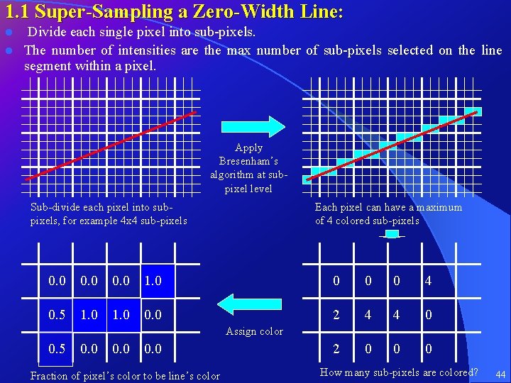
1. 1 Super-Sampling a Zero-Width Line: Divide each single pixel into sub-pixels. l The number of intensities are the max number of sub-pixels selected on the line segment within a pixel. l Apply Bresenham’s algorithm at subpixel level Sub-divide each pixel into subpixels, for example 4 x 4 sub-pixels Each pixel can have a maximum of 4 colored sub-pixels 0. 0 1. 0 0 4 0. 5 1. 0 0. 0 2 4 4 0 2 0 0 0 Assign color 0. 5 0. 0 Fraction of pixel’s color to be line’s color How many sub-pixels are colored? 44

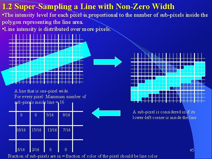
1. 2 Super-Sampling a Line with Non-Zero Width • The intensity level for each pixel is proportional to the number of sub-pixels inside the polygon representing the line area. • Line intensity is distributed over more pixels. A line that is one-pixel wide. For every pixel: Maximum number of sub-pixels inside line = 16 0 0 10/16 15/16 8/16 2/16 5/16 13/16 0 9/16 A sub-pixel is considered in if its lower-left corner is inside the line 7/16 0 Fraction of sub-pixels are in = fraction of color of the pixel should be line color 45

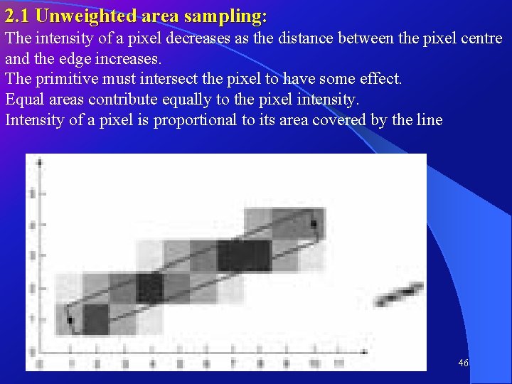
2. 1 Unweighted area sampling: The intensity of a pixel decreases as the distance between the pixel centre and the edge increases. The primitive must intersect the pixel to have some effect. Equal areas contribute equally to the pixel intensity. Intensity of a pixel is proportional to its area covered by the line 46

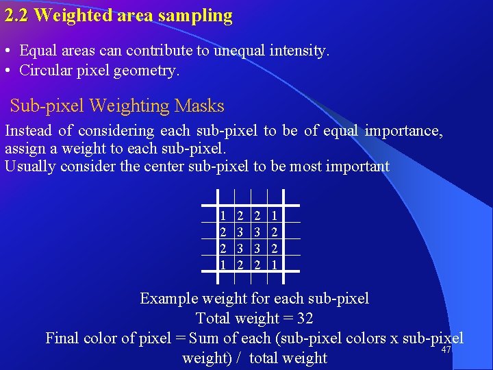
2. 2 Weighted area sampling • Equal areas can contribute to unequal intensity. • Circular pixel geometry. Sub-pixel Weighting Masks Instead of considering each sub-pixel to be of equal importance, assign a weight to each sub-pixel. Usually consider the center sub-pixel to be most important 1 2 2 1 2 3 3 2 1 2 2 1 Example weight for each sub-pixel Total weight = 32 Final color of pixel = Sum of each (sub-pixel colors x sub-pixel 47 weight) / total weight

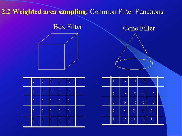
2. 2 Weighted area sampling: Common Filter Functions Box Filter Cone Filter 1 2 3 2 2 4 5 4 2 1 3 5 6 5 3 1 1 2 4 5 4 2 1 1 1 2 3 2 1 1 1 1 1 1

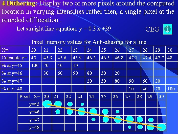
4 Dithering: Display two or more pixels around the computed location in varying intensities rather then, a single pixel at the rounded off location. Let straight line equation: y = 0. 3 x +39 CEG Pixel Intensity values for Anti-aliasing for a line X= 20 21 22 23 24 25 26 27 28 Calculate y= 45 45. 3 45. 6 45. 9 46. 2 46. 5 46. 8 47. 1 47. 4 47. 7 48 % at y=45 70 40 10 30 60 90 80 50 20 20 50 80 90 60 30 10 40 70 100 % at y=46 % at y=47 % at y=48 Pixel X= 20 21 y=45 y=46 y=47 y=48 22 23 24 25 26 27 28 29 29 30 30 100

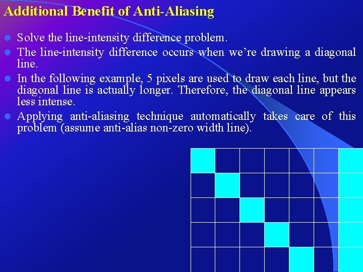
Additional Benefit of Anti-Aliasing Solve the line-intensity difference problem. The line-intensity difference occurs when we’re drawing a diagonal line. l In the following example, 5 pixels are used to draw each line, but the diagonal line is actually longer. Therefore, the diagonal line appears less intense. l Applying anti-aliasing technique automatically takes care of this problem (assume anti-alias non-zero width line). l l

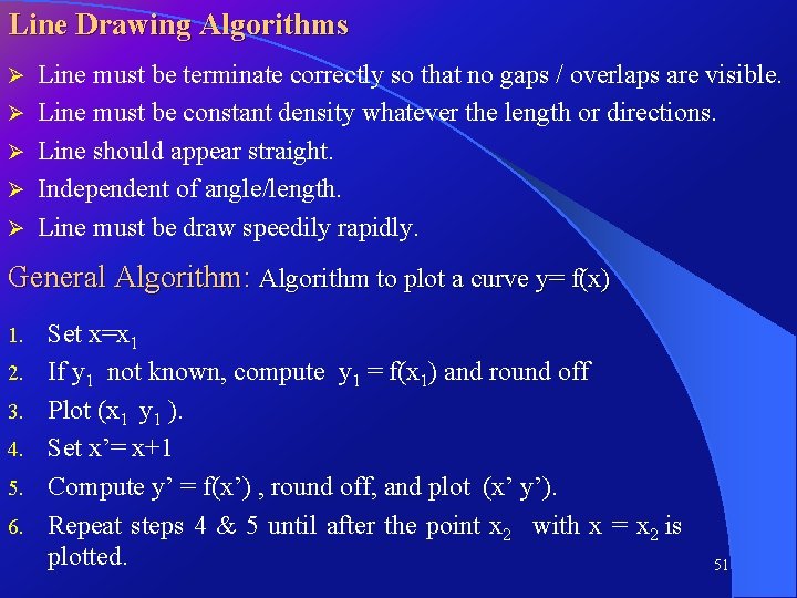
Line Drawing Algorithms Ø Ø Ø Line must be terminate correctly so that no gaps / overlaps are visible. Line must be constant density whatever the length or directions. Line should appear straight. Independent of angle/length. Line must be draw speedily rapidly. General Algorithm: Algorithm to plot a curve y= f(x) 1. 2. 3. 4. 5. 6. Set x=x 1 If y 1 not known, compute y 1 = f(x 1) and round off Plot (x 1 y 1 ). Set x’= x+1 Compute y’ = f(x’) , round off, and plot (x’ y’). Repeat steps 4 & 5 until after the point x 2 with x = x 2 is plotted. 51

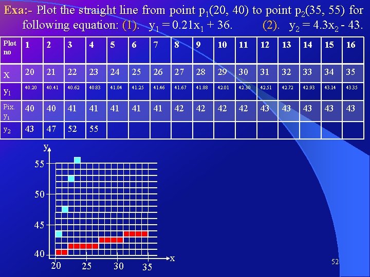
Exa: - Plot the straight line from point p 1(20, 40) to point p 2(35, 55) for following equation: (1). y 1 = 0. 21 x 1 + 36. (2). y 2 = 4. 3 x 2 - 43. Plot no 1 2 3 4 5 6 7 8 9 10 11 12 13 14 15 16 x 20 21 22 23 24 25 26 27 28 29 30 31 32 33 34 35 y 1 40. 20 40. 41 40. 62 40. 83 41. 04 41. 25 41. 46 41. 67 41. 88 42. 01 42. 30 42. 51 42. 72 42. 93 43. 14 43. 35 Pix. y 1 40 40 41 41 41 42 42 43 43 43 y 2 43 47 52 55 y 55 50 45 40 20 25 30 35 x 52

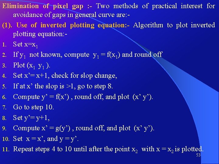
Elimination of pixel gap : - Two methods of practical interest for avoidance of gaps in general curve are: (1). Use of inverted plotting equation: - Algorithm to plot inverted plotting equation: 1. Set x=x 1 2. If y 1 not known, compute y 1 = f(x 1) and round off 3. Plot (x 1 y 1 ). 4. Set x’= x+1, check for slop change, 5. If at x’ the slop is >1, go to step 8. 6. Compute y’ = f(x’) , round off, and plot (x’ y’). 7. Go to step 10. 8. Set y’= y+1, 9. Compute x’ = g(y’) , round off, and plot (x’ y’). 10. Set x = x’, and y = y’. 11. Repeat steps 4 to 10 until after the point x 2 with x = x 2 is plotted. 53

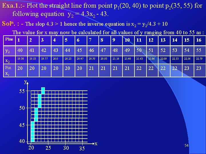
Exa. 1. : - Plot the straight line from point p 1(20, 40) to point p 2(35, 55) for following equation y 2 = 4. 3 x 2 - 43. Soln. : - The slop 4. 3 > 1 hence the inverse equation is x 2 = y 2/4. 3 + 10 The value for x may now be calculated for all values of y ranging from 40 to 55 as : Plno 1 2 3 4 5 6 7 8 9 10 11 12 13 14 15 16 y 2 40 41 42 43 44 45 46 47 48 49 50 51 52 53 54 55 x 2 19. 30 19. 53 19. 77 20. 0 20. 23 20. 47 20. 70 20. 93 21. 16 21. 40 21. 63 21. 86 22. 09 22. 33 22. 56 22. 79 Pix. 20 20 20 21 21 22 22 23 23 x 2 y 55 50 45 40 20 25 30 35 x 54

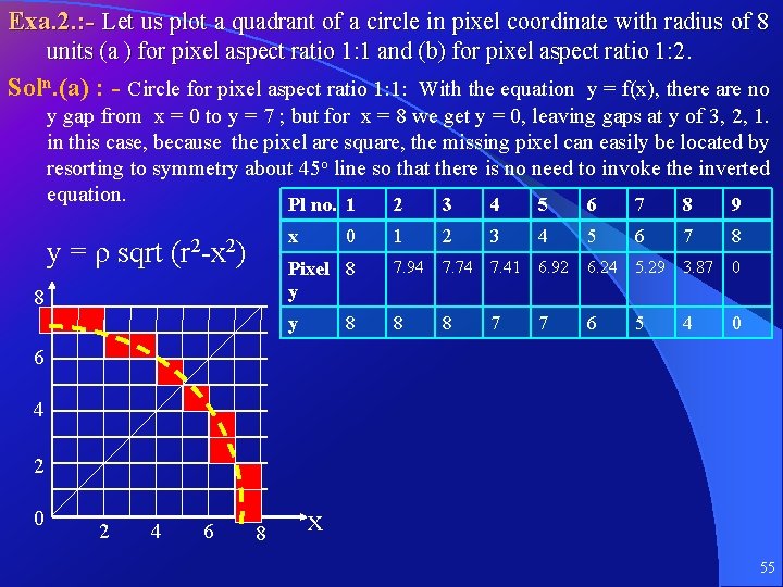
Exa. 2. : - Let us plot a quadrant of a circle in pixel coordinate with radius of 8 units (a ) for pixel aspect ratio 1: 1 and (b) for pixel aspect ratio 1: 2 Soln. (a) : - Circle for pixel aspect ratio 1: 1: With the equation y = f(x), there are no y gap from x = 0 to y = 7 ; but for x = 8 we get y = 0, leaving gaps at y of 3, 2, 1. in this case, because the pixel are square, the missing pixel can easily be located by resorting to symmetry about 45 o line so that there is no need to invoke the inverted equation. Pl no. 1 2 3 4 5 6 7 8 9 y = ρ sqrt x (r 2 -x 2) 8 0 1 2 3 4 5 6 7 8 Pixel 8 y 7. 94 7. 74 7. 41 6. 92 6. 24 5. 29 3. 87 0 y 8 8 7 7 6 5 4 0 8 6 4 2 0 2 4 6 8 x 55

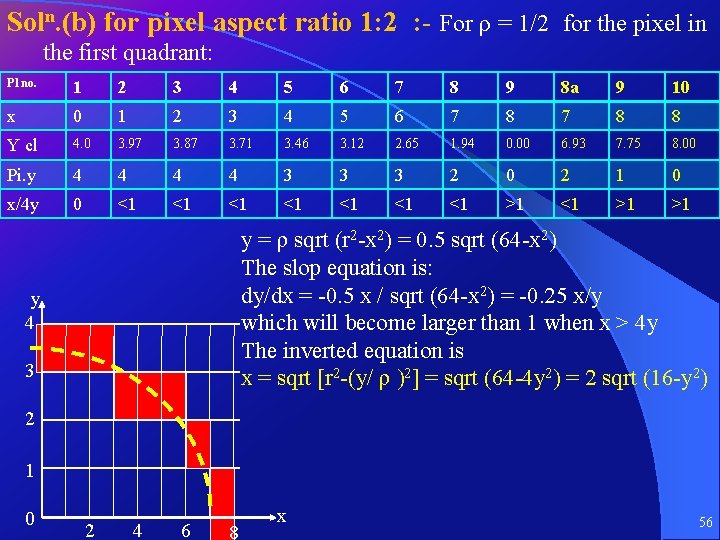
Soln. (b) for pixel aspect ratio 1: 2 : - For ρ = 1/2 for the pixel in the first quadrant: Pl no. 1 2 3 4 5 6 7 8 9 8 a 9 10 x 0 1 2 3 4 5 6 7 8 8 Y cl 4. 0 3. 97 3. 87 3. 71 3. 46 3. 12 2. 65 1. 94 0. 00 6. 93 7. 75 8. 00 Pi. y 4 4 3 3 3 2 0 2 1 0 x/4 y 0 <1 <1 >1 >1 y = ρ sqrt (r 2 -x 2) = 0. 5 sqrt (64 -x 2) The slop equation is: dy/dx = -0. 5 x / sqrt (64 -x 2) = -0. 25 x/y which will become larger than 1 when x > 4 y The inverted equation is x = sqrt [r 2 -(y/ ρ )2] = sqrt (64 -4 y 2) = 2 sqrt (16 -y 2) y 4 3 2 1 0 2 4 6 8 x 56

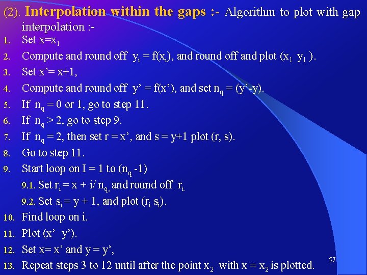
(2). Interpolation within the gaps : - Algorithm to plot with gap interpolation : 1. 2. 3. 4. 5. 6. 7. 8. 9. 10. 11. 12. 13. Set x=x 1 Compute and round off yi = f(xi), and round off and plot (x 1 y 1 ). Set x’= x+1, Compute and round off y’ = f(x’), and set nq = (y’-y). If nq = 0 or 1, go to step 11. If nq > 2, go to step 9. If nq = 2, then set r = x’, and s = y+1 plot (r, s). Go to step 11. Start loop on I = 1 to (nq -1) 9. 1. Set ri = x + i/ nq, and round off ri. 9. 2. Set si = y + 1, and plot (ri si). Find loop on i. Plot (x’ y’). Set x= x’ and y = y’, Repeat steps 3 to 12 until after the point x 2 with x = x 2 is plotted. 57

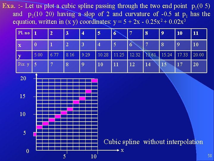
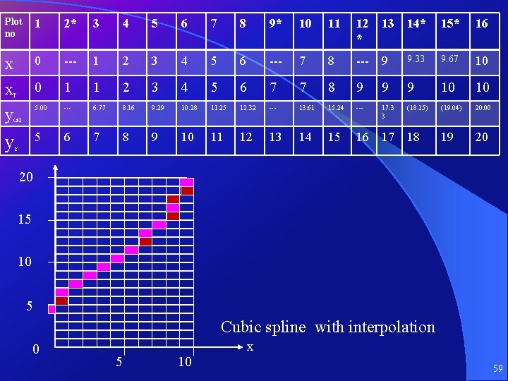
Exa. : - Let us plot a cubic spline passing through the two end point p 1(0 5) and p 2(10 20) having a slop of 2 and curvature of -0. 5 at p 1 has the equation, written in (x y) coordinates: y = 5 + 2 x - 0. 25 x 2 + 0. 02 x 3 Pl. no 1 2 3 4 5 6 7 8 9 10 11 x 0 1 2 3 4 5 6 7 8 9 10 y 5. 00 6. 77 8. 16 9. 29 10. 28 11. 25 12. 32 13. 61 15. 24 17. 33 20. 00 Pix. y 5 7 8 9 10 11 12 14 15 17 20 20 15 10 5 Cubic spline without interpolation 0 x 5 10 58

Plot no 1 2* 3 4 5 6 7 8 9* 10 11 12 * 13 14* 15* 16 x 0 --- 1 2 3 4 5 6 --- 7 8 --- 9 9. 33 9. 67 10 xr 0 1 1 2 3 4 5 6 7 7 8 9 9 9 10 10 y 5. 00 --- 6. 77 8. 16 9. 29 10. 28 11. 25 12. 32 --- 13. 61 15. 24 --- 17. 3 3 (18. 15) (19. 04) 20. 00 y 5 6 7 8 9 10 11 12 13 14 15 16 17 18 19 20 cal r 20 15 10 5 Cubic spline with interpolation 0 x 5 10 59

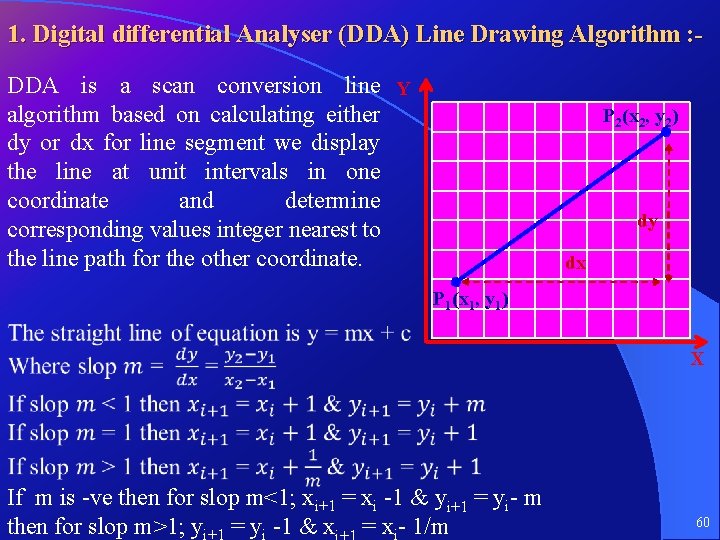
1. Digital differential Analyser (DDA) Line Drawing Algorithm : DDA is a scan conversion line Y algorithm based on calculating either dy or dx for line segment we display the line at unit intervals in one coordinate and determine corresponding values integer nearest to the line path for the other coordinate. P 2(x 2, y 2) dy dx P 1(x 1, y 1) X If m is -ve then for slop m<1; xi+1 = xi -1 & yi+1 = yi- m then for slop m>1; yi+1 = yi -1 & x = xi- 1/m 60

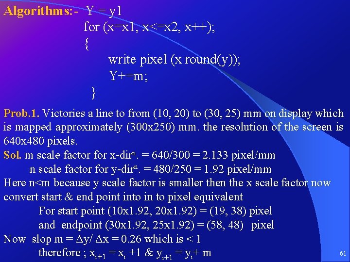
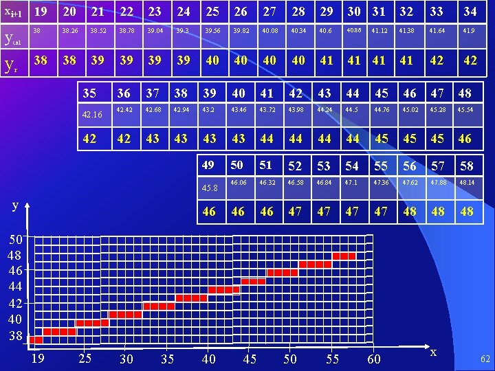
Algorithms: - Y = y 1 for (x=x 1, x<=x 2, x++); { write pixel (x round(y)); Y+=m; } Prob. 1. Victories a line to from (10, 20) to (30, 25) mm on display which is mapped approximately (300 x 250) mm. the resolution of the screen is 640 x 480 pixels. Sol. m scale factor for x-dirn. = 640/300 = 2. 133 pixel/mm n scale factor for y-dirn. = 480/250 = 1. 92 pixel/mm Here n<m because y scale factor is smaller then the x scale factor now convert start & end point into in to pixel equivalent For start point (10 x 1. 92, 20 x 1. 92) = (19, 38) pixel and endpoint (30 x 1. 92, 25 x 1. 92) = (58, 48) pixel Now slop m = Δy/ Δx = 0. 26 which is < 1 61 therefore ; xi+1 = xi +1 & yi+1 = yi+ m

xi+1 19 y 20 21 22 23 24 25 26 27 28 29 30 31 32 33 34 38 38. 26 38. 52 38. 78 39. 04 39. 3 39. 56 39. 82 40. 08 40. 34 40. 6 41. 38 41. 64 41. 9 38 38 39 39 40 40 41 41 42 42 36 37 38 39 40 41 42 43 44 45 46 47 48 42. 42 42. 68 42. 94 43. 2 43. 46 43. 72 43. 98 44. 24 44. 5 44. 76 45. 02 42 43 43 44 44 45 45 45 46 49 50 51 52 53 54 55 56 57 58 46. 06 46. 32 46. 58 46. 84 47. 1 47. 36 47. 62 47. 88 48. 14 46 46 47 47 48 48 48 40. 86 41. 12 cal y r 35 42. 16 42 45. 8 y 46 45. 28 45. 54 50 48 46 44 42 40 38 19 25 30 35 40 45 50 55 60 x 62

Prob. 1. To illustrate the DDA algorithm, digitise a line with P 1(18, 10) to P 2 (28, 15). Prob. 2. Scan convert the straight line with P 1(18, 8) to P 2 (25, 15). Prob. 3. , Digitise a line with P 1(18, 10) to P 2 (24, 25) To by DDA algorithm. Draw back: - 1. To find out every point, floating point addition and round off to integer. 2. More calculation time required. 63

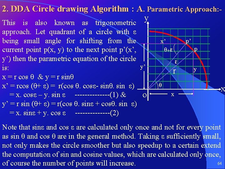
2. DDA Circle drawing Algorithm : A. Parametric Approach: y This is also known as trigonometric approach. Let quadrant of a circle with ε being small angle for shifting from the current point p(x, y) to the next point p’(x’, y’) then the parametric equation of the circle y’ is: x = r cos θ & y = r sinθ x’ = rcos (θ+ ε) = r(cos θ. cosε- sinθ. sin ε) = x. cosε – y. sin ε -------(1) & o y’ = r sin (θ+ ε) = r(cos θ. sinε + cosθ. sin ε) = x. sinε + y. cos ε -------(2) p’ x’ ᶿ+ᵋ p ᵋ r ᶿ x y x Note that sinε and cos ε are calculated only once and not for every point as sin θ and cos θ are in the general method. Taking ε sufficiently small, not only makes the circle smoother but also speedup to a certain extend the computation of sin and cosine values, which are calculated only once, 64 of course the number of points will increase.

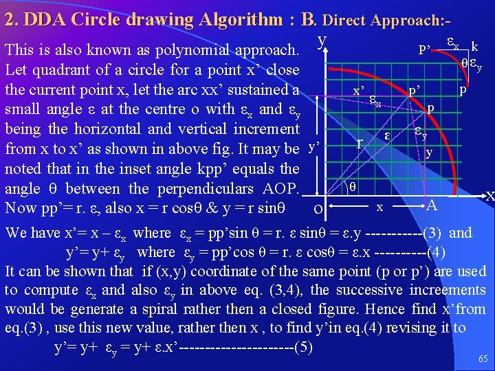
2. DDA Circle drawing Algorithm : B. Direct Approach: εx y P’ This is also known as polynomial approach. Let quadrant of a circle for a point x’ close the current point x, let the arc xx’ sustained a small angle ε at the centre o with εx and εy being the horizontal and vertical increment from x to x’ as shown in above fig. It may be y’ noted that in the inset angle kpp’ equals the angle θ between the perpendiculars AOP. Now pp’= r. ε, also x = r cosθ & y = r sinθ o x’ ᶿ p ᵋ r x ᶿ εy p p’ εx k εy y x A We have x’= x – εx where εx = pp’sin θ = r. ε sinθ = ε. y ------(3) and y’= y+ εy where εy = pp’cos θ = r. ε cosθ = ε. x -----(4) It can be shown that if (x, y) coordinate of the same point (p or p’) are used to compute εx and also εy in above eq. (3, 4), the successive increements would be generate a spiral rather then a closed figure. Hence find x’from eq. (3) , use this new value, rather then x , to find y’in eq. (4) revising it to y’= y+ εy = y+ ε. x’-----------(5) 65

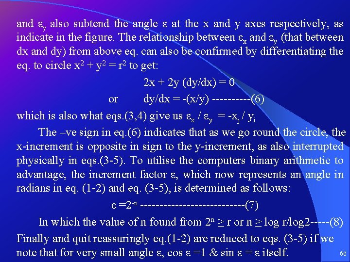
and εy also subtend the angle ε at the x and y axes respectively, as indicate in the figure. The relationship between εx and εy (that between dx and dy) from above eq. can also be confirmed by differentiating the eq. to circle x 2 + y 2 = r 2 to get: 2 x + 2 y (dy/dx) = 0 or dy/dx = -(x/y) -----(6) which is also what eqs. (3, 4) give us εx / εy = -xj / yi The –ve sign in eq. (6) indicates that as we go round the circle, the x-increment is opposite in sign to the y-increment, as also interrupted physically in eqs. (3 -5). To utilise the computers binary arithmetic to advantage, the increment factor ε, which now represents an angle in radians in eq. (1 -2) and eq. (3 -5), is determined as follows: ε =2 -n --------------(7) In which the value of n found from 2 n ≥ r or n ≥ log r/log 2 -----(8) Finally and quit reassuringly eq. (1 -2) are reduced to eqs. (3 -5) if we 66 note that for very small angle ε, cos ε =1 & sin ε = ε itself.

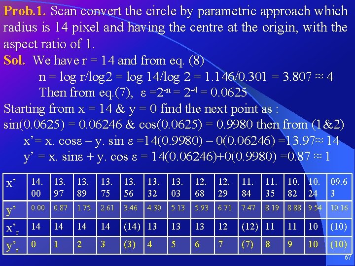
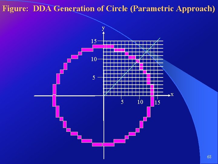
Prob. 1. Scan convert the circle by parametric approach which radius is 14 pixel and having the centre at the origin, with the aspect ratio of 1. Sol. We have r = 14 and from eq. (8) n = log r/log 2 = log 14/log 2 = 1. 146/0. 301 = 3. 807 ≈ 4 Then from eq. (7), ε =2 -n = 2 -4 = 0. 0625 Starting from x = 14 & y = 0 find the next point as : sin(0. 0625) = 0. 06246 & cos(0. 0625) = 0. 9980 then from (1&2) x’= x. cosε – y. sin ε =14(0. 9980) – 0(0. 06246) =13. 97≈ 14 y’ = x. sinε + y. cos ε = 14(0. 06246)+0(0. 9980) =0. 87 ≈ 1 x’ 14. 00 13. 97 13. 89 13. 75 13. 56 13. 32 13. 03 12. 68 12. 29 11. 84 11. 35 10. 82 24 09. 6 3 y’ x’r y’r 0. 00 0. 87 1. 75 2. 61 3. 46 4. 30 5. 13 5. 93 6. 71 7. 47 8. 19 8. 88 9. 54 10. 16 14 14 (14) 13 13 13 12 (12) 11 11 10 (10) 0 1 2 3 (3) 5 6 7 (7) 9 10 (10) 4 8 67

Figure: DDA Generation of Circle (Parametric Approach) y 15 10 5 x 5 10 15 68

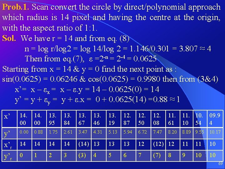
Prob. 1. Scan convert the circle by direct/polynomial approach which radius is 14 pixel and having the centre at the origin, with the aspect ratio of 1: 1. Sol. We have r = 14 and from eq. (8) n = log r/log 2 = log 14/log 2 = 1. 146/0. 301 = 3. 807 ≈ 4 Then from eq. (7), ε =2 -n = 2 -4 = 0. 0625 Starting from x = 14 & y = 0 find the next point as : sin(0. 0625) = 0. 06246 & cos(0. 0625) = 0. 9980 then from (3&4) x’= x – εx = x – ε. y = 14 – 0. 0625(0) = 14 y’ = y + εy = y + ε. x = 0 + 0. 0625(14) =0. 88 ≈ 1 x’ 14. 00 13. 95 13. 84 13. 67 13. 46 13. 19 12. 87 12. 50 12. 08 11. 61 11. 10 54 09. 9 4 y’ x’r y’r 0. 00 0. 88 1. 75 2. 61 3. 47 4. 31 5. 13 5. 94 6. 72 7. 47 8. 20 8. 89 9. 55 10. 17 14 14 (14) 13 13 13 12 (12) 12 11 11 10 0 1 2 3 (3) 5 6 7 (7) 9 10 10 4 8 69

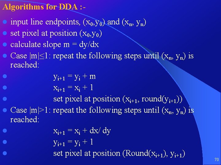
Algorithms for DDA : l l l input line endpoints, (x 0, y 0) and (xn, yn) set pixel at position (x 0, y 0) calculate slope m = dy/dx Case |m|≤ 1: repeat the following steps until (xn, yn) is reached: yi+1 = yi + m xi+1 = xi + 1 set pixel at position (xi+1, round(yi+1)) Case |m|>1: repeat the following steps until (xn, yn) is reached: xi+1 = xi + dx/ dy yi+1 = yi + 1 set pixel at position (Round(xi+1), yi+1) 70

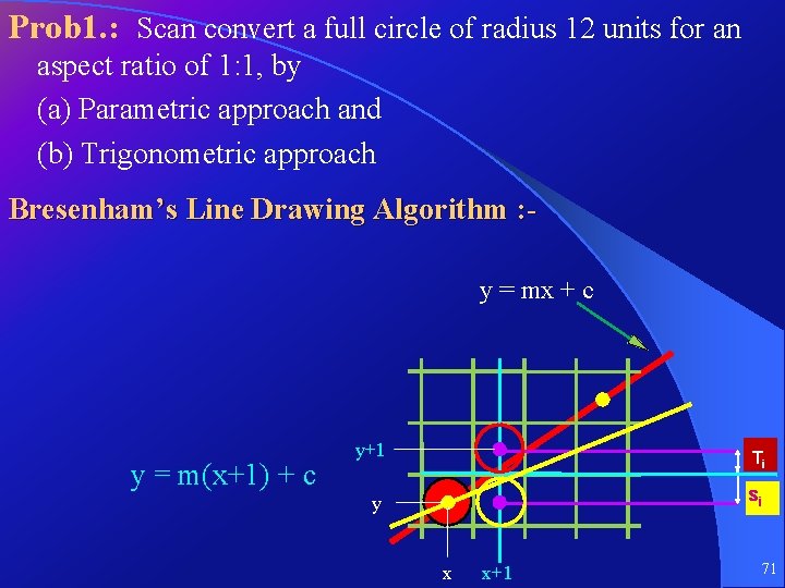
Prob 1. : Scan convert a full circle of radius 12 units for an aspect ratio of 1: 1, by (a) Parametric approach and (b) Trigonometric approach Bresenham’s Line Drawing Algorithm : y = mx + c y = m(x+1) + c y+1 Ti si y x x+1 71

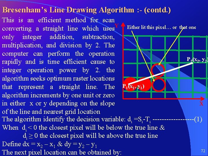
Bresenham’s Line Drawing Algorithm : - (contd. ) This is an efficient method for scan converting a straight line which uses. Y Either lit this pixel… or that one only integer addition, subtraction, multiplication, and division by 2. The computer can perform the operation P 2(x 2, y 2) rapidly and is time efficient cause to integer operation power by 2. the algorithm seeks optimum raster locations that represent a straight line. The PP 1(x 1, 1, yy 1)1) 1(x algorithm increments by one unit or zero X in either x or y depending on the slope of the line and nearest grid location The algorithm identify the decision variable: di =Si-Ti ---------(1) When di < 0 the closest pixel will be below the true line & di ≥ 0 the closest pixel will be above the true line Define dx = x 2 – x 1 & dy = y 2 – y 1 72 The next pixel location can be obtained by:

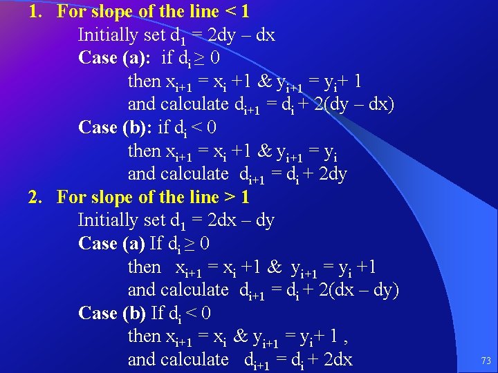
1. For slope of the line < 1 Initially set d 1 = 2 dy – dx Case (a): if di ≥ 0 then xi+1 = xi +1 & yi+1 = yi+ 1 and calculate di+1 = di + 2(dy – dx) Case (b): if di < 0 then xi+1 = xi +1 & yi+1 = yi and calculate di+1 = di + 2 dy 2. For slope of the line > 1 Initially set d 1 = 2 dx – dy Case (a) If di ≥ 0 then xi+1 = xi +1 & yi+1 = yi +1 and calculate di+1 = di + 2(dx – dy) Case (b) If di < 0 then xi+1 = xi & yi+1 = yi+ 1 , and calculate di+1 = di + 2 dx 73

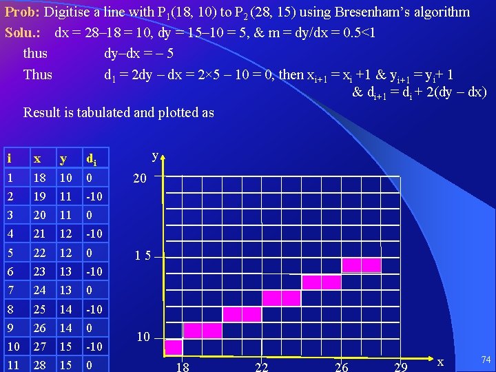
Prob: Digitise a line with P 1(18, 10) to P 2 (28, 15) using Bresenham’s algorithm Solu. : dx = 28– 18 = 10, dy = 15– 10 = 5, & m = dy/dx = 0. 5<1 thus dy–dx = – 5 Thus d 1 = 2 dy – dx = 2× 5 – 10 = 0, then xi+1 = xi +1 & yi+1 = yi+ 1 & di+1 = di + 2(dy – dx) Result is tabulated and plotted as i x y di 1 18 10 0 2 19 11 -10 3 20 11 0 4 21 12 -10 5 22 12 0 6 23 13 -10 7 24 13 0 8 25 14 -10 9 26 14 0 10 27 15 -10 11 28 15 0 y 20 15 10 x 74

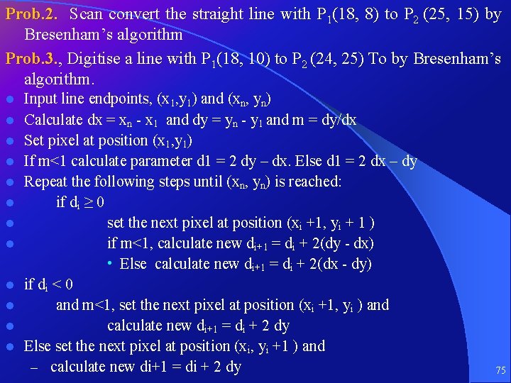
Prob. 2. Scan convert the straight line with P 1(18, 8) to P 2 (25, 15) by Bresenham’s algorithm Prob. 3. , Digitise a line with P 1(18, 10) to P 2 (24, 25) To by Bresenham’s algorithm. l l l Input line endpoints, (x 1, y 1) and (xn, yn) Calculate dx = xn - x 1 and dy = yn - y 1 and m = dy/dx Set pixel at position (x 1, y 1) If m<1 calculate parameter d 1 = 2 dy – dx. Else d 1 = 2 dx – dy Repeat the following steps until (xn, yn) is reached: if di ≥ 0 set the next pixel at position (xi +1, yi + 1 ) if m<1, calculate new di+1 = di + 2(dy - dx) • Else calculate new di+1 = di + 2(dx - dy) if di < 0 and m<1, set the next pixel at position (xi +1, yi ) and calculate new di+1 = di + 2 dy Else set the next pixel at position (xi, yi +1 ) and – calculate new di+1 = di + 2 dy 75

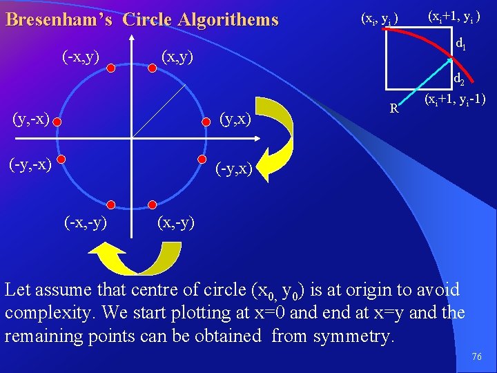
Bresenham’s Circle Algorithems (-x, y) (xi, yi ) (xi+1, yi ) d 1 (x, y) d 2 (y, -x) (y, x) (-y, -x) (-y, x) (-x, -y) R (xi+1, yi-1) (x, -y) Let assume that centre of circle (x 0, y 0) is at origin to avoid complexity. We start plotting at x=0 and end at x=y and the remaining points can be obtained from symmetry. 76

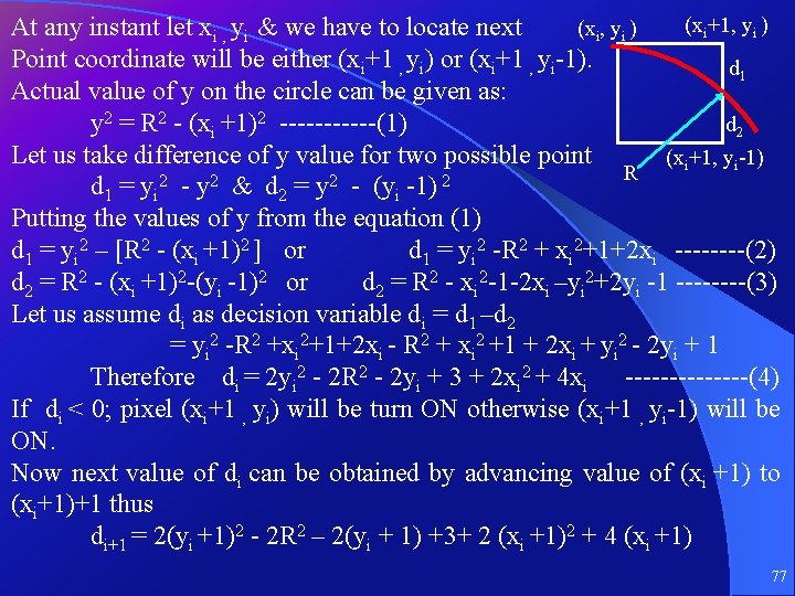
(xi+1, yi ) (xi, yi ) At any instant let xi , yi & we have to locate next Point coordinate will be either (xi+1 , yi) or (xi+1 , yi-1). d 1 Actual value of y on the circle can be given as: d 2 y 2 = R 2 - (xi +1)2 ------(1) Let us take difference of y value for two possible point (xi+1, yi-1) R d 1 = yi 2 - y 2 & d 2 = y 2 - (yi -1) 2 Putting the values of y from the equation (1) d 1 = yi 2 – [R 2 - (xi +1)2 ] or d 1 = yi 2 -R 2 + xi 2+1+2 xi ----(2) d 2 = R 2 - (xi +1)2 -(yi -1)2 or d 2 = R 2 - xi 2 -1 -2 xi –yi 2+2 yi -1 ----(3) Let us assume di as decision variable di = d 1 –d 2 = yi 2 -R 2 +xi 2+1+2 xi - R 2 + xi 2 +1 + 2 xi + yi 2 - 2 yi + 1 Therefore di = 2 yi 2 - 2 R 2 - 2 yi + 3 + 2 xi 2 + 4 xi -------(4) If di < 0; pixel (xi+1 , yi) will be turn ON otherwise (xi+1 , yi-1) will be ON. Now next value of di can be obtained by advancing value of (xi +1) to (xi+1)+1 thus di+1 = 2(yi +1)2 - 2 R 2 – 2(yi + 1) +3+ 2 (xi +1)2 + 4 (xi +1) 77

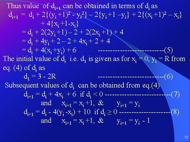
Thus value of di+1 can be obtained in terms of di as di+1 = di + 2{(yi +1)2 - yi 2} – 2{yi +1 –yi} + 2{(xi +1)2 – xi} + 4{xi +1 -xi} = di + 2(2 yi +1) – 2 + 2(2 xi +1) + 4 = di + 4 yi + 2 – 2 + 4 xi + 2 + 4 = di + 4(xi +yi) + 6 --------------(5) The initial value of di i. e. d 1 is given as for xi = 0, yi = R from eq. (4) of di as d 1 = 3 - 2 R --------------(6) Subsequent values of di can be obtained from eq. (4) di+1 = di + 4 xi + 6 if di < 0 --------------(7) and xi+1 = xi +1, & yi+1 = yi di+1 = di - 4(yi -xi) + 10 if di ≥ 0 -----------(8) and xi+1 = xi +1, & yi+1 = yi - 1 78

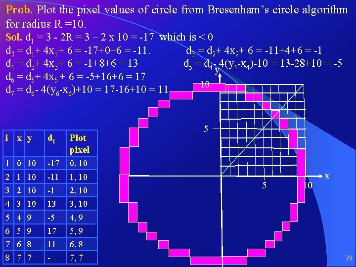
Prob. Plot the pixel values of circle from Bresenham’s circle algorithm for radius R =10. Sol. d 1 = 3 - 2 R = 3 – 2 x 10 = -17 which is < 0 d 2 = d 1+ 4 x 1+ 6 = -17+0+6 = -11. d 3 = d 2+ 4 x 2+ 6 = -11+4+6 = -1 d 4 = d 3+ 4 x 3+ 6 = -1+8+6 = 13 d 5 = d 4 - 4(y 4 -x 4)-10 = 13 -28+10 = -5 y d 6 = d 5+ 4 x 5 + 6 = -5+16+6 = 17 10 d 7 = d 6 - 4(y 6 -x 6)+10 = 17 -16+10 = 11 i x y di Plot pixel 1 0 10 -17 0, 10 2 1 10 -11 1, 10 3 2 10 -1 2, 10 4 3 10 13 3, 10 5 4 9 -5 4, 9 6 5 9 17 5, 9 7 6 8 11 6, 8 8 7 7 - 7, 7 5 5 10 x 79

Prob. 1. Scan convert the circle from Bresenham’s circle algorithm which radius is 14 pixel. Prob. 2. Scan convert one quadrant of a circle of radius 10 units by the Bresenham’s algorithm. Prob. 3. Plot one quadrant of a circle of radius 7 units by the Bresenham’s algorithm with the origin at the centre. 80

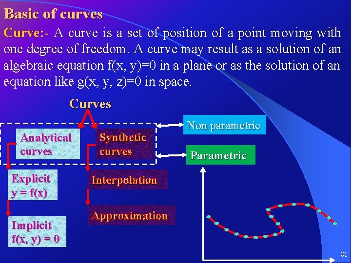
Basic of curves Curve: - A curve is a set of position of a point moving with one degree of freedom. A curve may result as a solution of an algebraic equation f(x, y)=0 in a plane or as the solution of an equation like g(x, y, z)=0 in space. Curves Analytical curves Explicit y = f(x) Implicit f(x, y) = 0 Synthetic curves Non parametric Parametric Interpolation Approximation 81

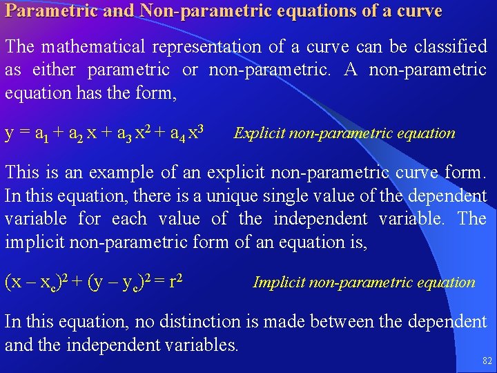
Parametric and Non-parametric equations of a curve The mathematical representation of a curve can be classified as either parametric or non-parametric. A non-parametric equation has the form, y = a 1 + a 2 x + a 3 x 2 + a 4 x 3 Explicit non-parametric equation This is an example of an explicit non-parametric curve form. In this equation, there is a unique single value of the dependent variable for each value of the independent variable. The implicit non-parametric form of an equation is, (x – xc)2 + (y – yc)2 = r 2 Implicit non-parametric equation In this equation, no distinction is made between the dependent and the independent variables. 82

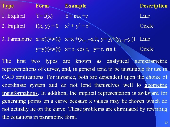
Type Form Example Description 1. Explicit Y= f(x) Y= mx +c Line 2. Implicit f(x, y) = 0 x 2 + y 2 = r 2 Circle 3. Parametric x=x(t)/w(t) x=xi+(xi+1–xi)t, y= yi+(yi+1–yi)t Line y=y(t)/w(t) x= r. cos t; y= r. sin t Circle The first two types are known as analytical nonparametric representations of curves, and, in general tend to be unsuitable for use in CAD applications. For instance, both are dependent upon the choice of coordinate system and do not lend themselves well to geometric transformations. In addition, the implicit representation is awkward for generating points on a curve because x values may be chosen which do not actually lie on the curve. These problems are eliminated by rewriting the equations in parametric form. 83

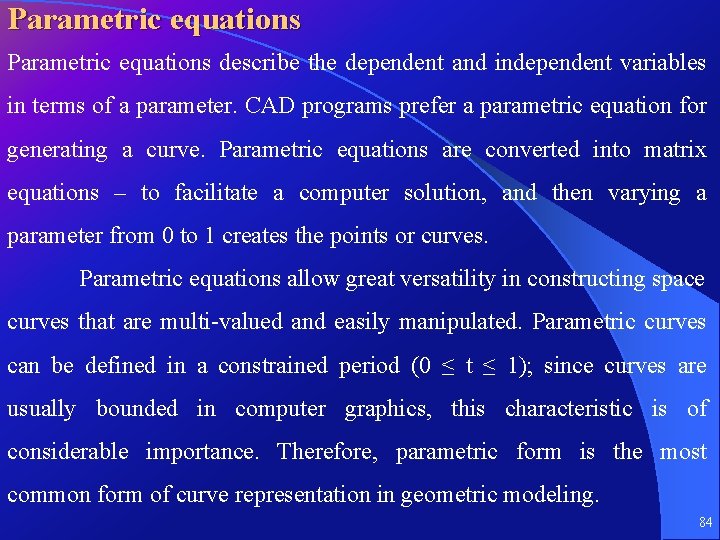
Parametric equations describe the dependent and independent variables in terms of a parameter. CAD programs prefer a parametric equation for generating a curve. Parametric equations are converted into matrix equations – to facilitate a computer solution, and then varying a parameter from 0 to 1 creates the points or curves. Parametric equations allow great versatility in constructing space curves that are multi-valued and easily manipulated. Parametric curves can be defined in a constrained period (0 ≤ t ≤ 1); since curves are usually bounded in computer graphics, this characteristic is of considerable importance. Therefore, parametric form is the most common form of curve representation in geometric modeling. 84

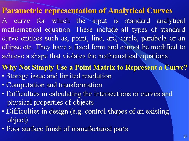
Parametric representation of Analytical Curves A curve for which the input is standard analytical mathematical equation. These include all types of standard curve entities such as, point, line, arc, circle, parabola or an ellipse etc. They have a fixed form and cannot be modified to achieve a shape that violates the mathematical equations. Why Not Simply Use a Point Matrix to Represent a Curve? • Storage issue and limited resolution • Computation and transformation • Difficulties in calculating the intersections or curves and physical properties of objects • Difficulties in design (e. g. control shapes of an existing object) • Poor surface finish of manufactured parts 85

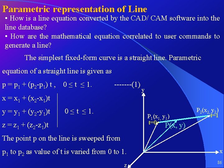
Parametric representation of Line • How is a line equation converted by the CAD/ CAM software into the line database? • How are the mathematical equation correlated to user commands to generate a line? The simplest fixed-form curve is a straight line. Parametric equation of a straight line is given as p = p 1 + (p 2 -p 1) t , 0 ≤ t ≤ 1. -------(1) y x = x 1 + (x 2 -x 1)t y = y 1 + (y 2 -y 1)t 0 ≤ t ≤ 1. P 1(x 1, y 1) t=0 z = z 1 + (z 2 -z 1)t P 2(x 2, y 2) t=1 P(x, y) The point p on the line is sweeped from p 1 to p 2 as value of t is varied from 0 to 1. x z 86

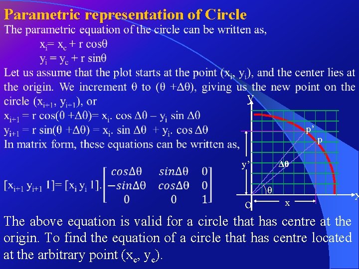
Parametric representation of Circle y p’ y’ p Δθ ᶿ o The above equation is valid for a circle that has centre at the origin. To find the equation of a circle that has centre located at the arbitrary point (xc, yc). x x

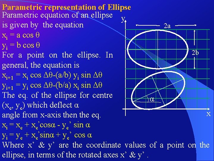
Parametric representation of Ellipse Parametric equation of an ellipse y is given by the equation 2 a xi = a cos θ yi = b cos θ 2 b For a point on the ellipse. In general, the equation is xi+1 = xi cos Δθ-(a/b) yi sin Δθ yi+1 = yi cos Δθ-(b/a) xi sin Δθ The eq. of the ellipse for centre α (xc, yc) which deflect α x angle from x-axis then the eq. xi = xc + xc’cosα - yc’ sin α yi = yc + xc’sinα + yc’ cos α Where x’ & y’ are the coordinate values of a point on the ellipse, in terms of the rotated axes x’ & y’.

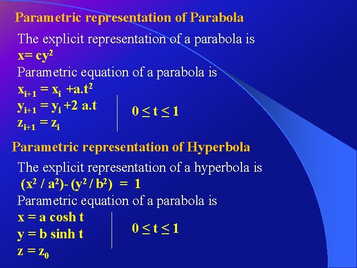
Parametric representation of Parabola The explicit representation of a parabola is x= cy 2 Parametric equation of a parabola is xi+1 = xi +a. t 2 yi+1 = yi +2 a. t 0≤t≤ 1 zi+1 = zi Parametric representation of Hyperbola The explicit representation of a hyperbola is (x 2 / a 2)- (y 2 / b 2) = 1 Parametric equation of a parabola is x = a cosh t 0≤t≤ 1 y = b sinh t z = z 0

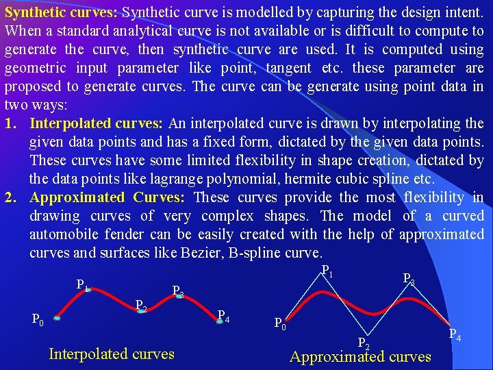
Synthetic curves: Synthetic curve is modelled by capturing the design intent. When a standard analytical curve is not available or is difficult to compute to generate the curve, then synthetic curve are used. It is computed using geometric input parameter like point, tangent etc. these parameter are proposed to generate curves. The curve can be generate using point data in two ways: 1. Interpolated curves: An interpolated curve is drawn by interpolating the given data points and has a fixed form, dictated by the given data points. These curves have some limited flexibility in shape creation, dictated by the data points like lagrange polynomial, hermite cubic spline etc. 2. Approximated Curves: These curves provide the most flexibility in drawing curves of very complex shapes. The model of a curved automobile fender can be easily created with the help of approximated curves and surfaces like Bezier, B-spline curve. P 1 P 0 P 2 P 3 Interpolated curves P 4 P 0 P 2 Approximated curves P 4

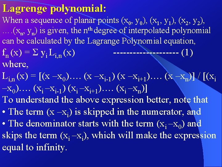
Lagrenge polynomial: When a sequence of planar points (x 0, y 0), (x 1, y 1), (x 2, y 2), …. (xn, yn) is given, the nth degree of interpolated polynomial can be calculated by the Lagrange Polynomial equation, fn (x) = Σ yi Li, n (x) ---------- (1) where, Li, n (x) = [(x –x 0)…. (x –xi-1) (x –xi+1)…. (x –xn)] / [(xi –x 0)…. (xi –xi-1) (xi –xi+1)…. (xi –xn)] To understand the above expression better, note that • The term (x –xi) is skipped in the numerator, and • The denominator starts with the term (xi –x 0) and skips the term (xi –xi), which will make the expression equal to infinity.

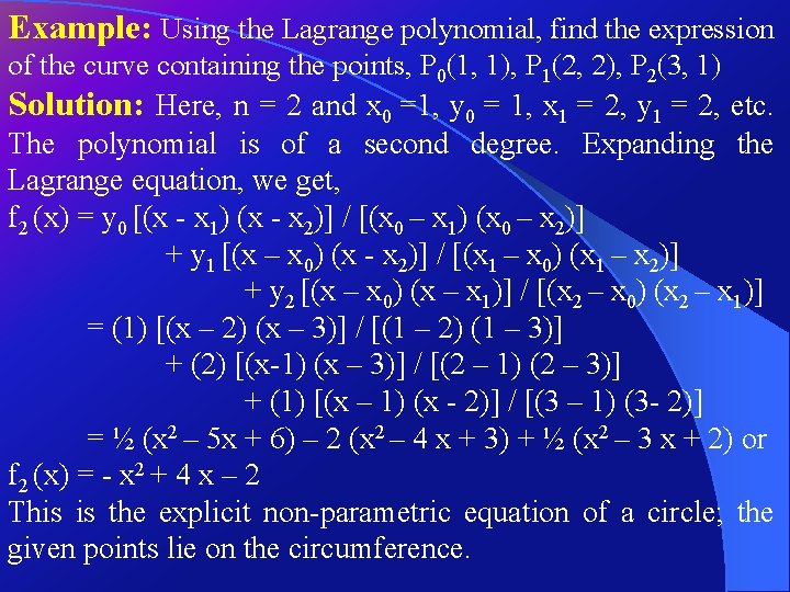
Example: Using the Lagrange polynomial, find the expression of the curve containing the points, P 0(1, 1), P 1(2, 2), P 2(3, 1) Solution: Here, n = 2 and x 0 =1, y 0 = 1, x 1 = 2, y 1 = 2, etc. The polynomial is of a second degree. Expanding the Lagrange equation, we get, f 2 (x) = y 0 [(x - x 1) (x - x 2)] / [(x 0 – x 1) (x 0 – x 2)] + y 1 [(x – x 0) (x - x 2)] / [(x 1 – x 0) (x 1 – x 2)] + y 2 [(x – x 0) (x – x 1)] / [(x 2 – x 0) (x 2 – x 1)] = (1) [(x – 2) (x – 3)] / [(1 – 2) (1 – 3)] + (2) [(x-1) (x – 3)] / [(2 – 1) (2 – 3)] + (1) [(x – 1) (x - 2)] / [(3 – 1) (3 - 2)] = ½ (x 2 – 5 x + 6) – 2 (x 2 – 4 x + 3) + ½ (x 2 – 3 x + 2) or f 2 (x) = - x 2 + 4 x – 2 This is the explicit non-parametric equation of a circle; the given points lie on the circumference.

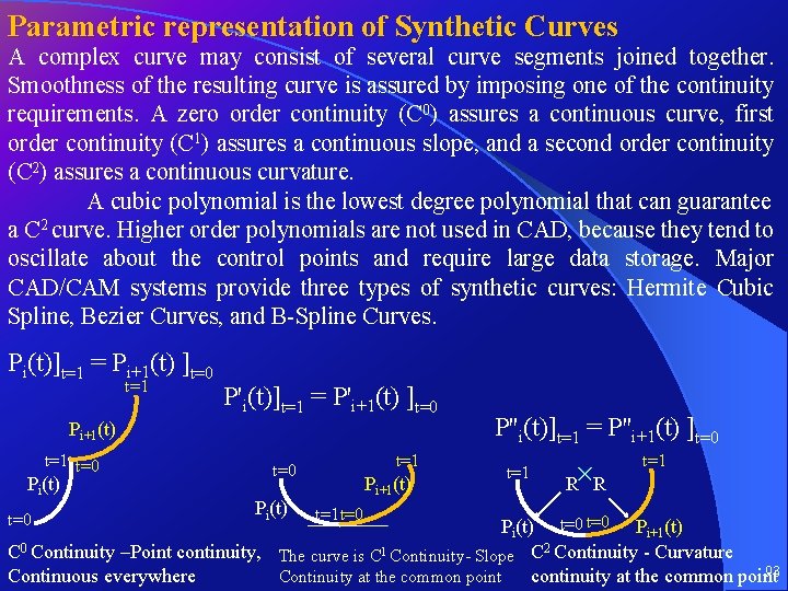
Parametric representation of Synthetic Curves A complex curve may consist of several curve segments joined together. Smoothness of the resulting curve is assured by imposing one of the continuity requirements. A zero order continuity (C 0) assures a continuous curve, first order continuity (C 1) assures a continuous slope, and a second order continuity (C 2) assures a continuous curvature. A cubic polynomial is the lowest degree polynomial that can guarantee a C 2 curve. Higher order polynomials are not used in CAD, because they tend to oscillate about the control points and require large data storage. Major CAD/CAM systems provide three types of synthetic curves: Hermite Cubic Spline, Bezier Curves, and B-Spline Curves. Pi(t)]t=1 = Pi+1(t) ]t=0 t=1 P'i(t)]t=1 = P'i+1(t) ]t=0 Pi+1(t) t=1 t=0 Pi(t) t=0 t=1 t=0 Pi(t) Pi+1(t) t=1 t=0 P''i(t)]t=1 = P''i+1(t) ]t=0 t=1 R R Pi(t) t=0 Pi+1(t) C 0 Continuity –Point continuity, The curve is C 1 Continuity- Slope C 2 Continuity - Curvature 93 Continuous everywhere continuity at the common point Continuity at the common point

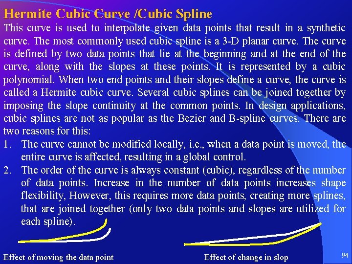
Hermite Cubic Curve /Cubic Spline This curve is used to interpolate given data points that result in a synthetic curve. The most commonly used cubic spline is a 3 -D planar curve. The curve is defined by two data points that lie at the beginning and at the end of the curve, along with the slopes at these points. It is represented by a cubic polynomial. When two end points and their slopes define a curve, the curve is called a Hermite cubic curve. Several cubic splines can be joined together by imposing the slope continuity at the common points. In design applications, cubic splines are not as popular as the Bezier and B-spline curves. There are two reasons for this: 1. The curve cannot be modified locally, i. e. , when a data point is moved, the entire curve is affected, resulting in a global control. 2. The order of the curve is always constant (cubic), regardless of the number of data points. Increase in the number of data points increases shape flexibility, However, this requires more data points, creating more splines, that are joined together (only two data points and slopes are utilized for each spline). Effect of moving the data point Effect of change in slop 94

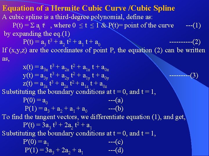
Equation of a Hermite Cubic Curve /Cubic Spline A cubic spline is a third-degree polynomial, define as: P(t) = Σ ai ti , where 0 ≤ t ≤ 1 & P(t)= point of the curve ---(1) by expanding the eq. (1) P(t) = a 3 t 3 + a 2 t 2 + a 1 t + a 0 -----(2) If (x, y, z) are the coordinates of point P, the equation (2) can be written as, x(t) = a 3 x t 3 + a 2 x t 2 + a 1 x t + a 0 x y(t) = a 3 y t 3 + a 2 y t 2 + a 1 y t + a 0 y -----(3) z(t) = a 3 z t 3 + a 2 z t 2 + a 1 z t + a 0 z Substituting the boundary conditions at t = 0, and t = 1, P(0) = a 0 ---(a) P(1) = a 3 + a 2 + a 1 + a 0 ---(b) To find the tangent vectors, we differentiate equation (1), and get, P'(t) = 3 a 3 t 3 + 2 a 2 t 2 + a 1 Substituting the boundary conditions at t = 0, and t = 1, P'(0) = a 1 ---(c) P'(1) = 3 a 3 + 2 a 2 + a 1 ---(d)

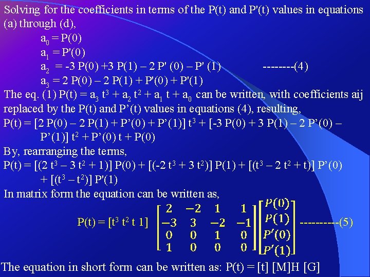
Solving for the coefficients in terms of the P(t) and P'(t) values in equations (a) through (d), a 0 = P(0) a 1 = P'(0) a 2 = -3 P(0) +3 P(1) – 2 P' (0) – P' (1) ----(4) a 3 = 2 P(0) – 2 P(1) + P'(0) + P'(1) The eq. (1) P(t) = a 3 t 3 + a 2 t 2 + a 1 t + a 0 can be written, with coefficients aij replaced by the P(t) and P’(t) values in equations (4), resulting, P(t) = [2 P(0) – 2 P(1) + P’(0) + P’(1)] t 3 + [-3 P(0) + 3 P(1) – 2 P’(0) – P’(1)] t 2 + P’(0) t + P(0) By, rearranging the terms, P(t) = [(2 t 3 – 3 t 2 + 1)] P(0) + [(-2 t 3 + 3 t 2)] P(1) + [(t 3 – 2 t 2 + t)] P’(0) + [(t 3 – t 2)] P'(1) In matrix form the equation can be written as, P(t) = [t 3 t 2 t 1] -----(5) The equation in short form can be written as: P(t) = [t] [M]H [G]

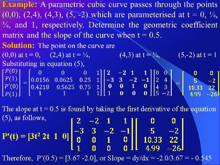
The slope at t = 0. 5 is found by taking the first derivative of the equation (5), as follows, P'(t) = [3 t 2 2 t 1 0] Therefore, P’(0. 5) = [3. 67 -2. 0], or Slope = dy/dx = -2. 0/3. 67 = - 0. 545

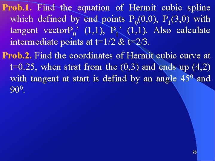
Prob. 1. Find the equation of Hermit cubic spline which defined by end points P 0(0, 0), P 1(3, 0) with tangent vector. P 0’ (1, 1), P 1’ (1, 1). Also calculate intermediate points at t=1/2 & t=2/3. Prob. 2. Find the coordinates of Hermit cubic curve at t=0. 25, when strat from the (0, 3) and ends up (4, 2) with tangent at start is defind by an angle 450 and 900. 98

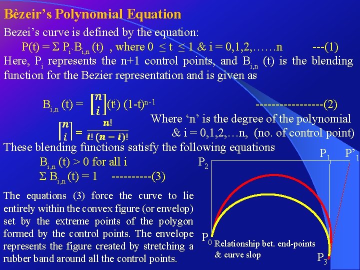
Bèzeir’s Polynomial Equation Bezei’s curve is defined by the equation: P(t) = Σ Pi`Bi, n (t) , where 0 ≤ t ≤ 1 & i = 0, 1, 2, ……n ---(1) Here, Pi represents the n+1 control points, and Bi, n (t) is the blending function for the Bezier representation and is given as Bi, n (t) = (ti) (1 -t)n-1 ---------(2) Where ‘n’ is the degree of the polynomial = & i = 0, 1, 2, …n, (no. of control point) These blending functions satisfy the following equations P 1 P’ 1 P 2 Bi, n (t) > 0 for all i Σ Bi, n (t) = 1 -----(3) The equations (3) force the curve to lie entirely within the convex figure (or envelop) set by the extreme points of the polygon formed by the control points. The envelope P represents the figure created by stretching a 0 Relationship bet. end-points & curve slop P 3 rubber band around all the control points.

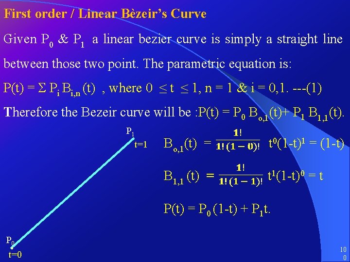
First order / Linear Bèzeir’s Curve Given P 0 & P 1 a linear bezier curve is simply a straight line between those two point. The parametric equation is: P(t) = Σ Pi Bi, n (t) , where 0 ≤ t ≤ 1, n = 1 & i = 0, 1. ---(1) Therefore the Bezeir curve will be : P(t) = P 0 Bo, 1(t)+ P 1 B 1, 1(t). P 1 t=1 Bo, 1(t) = t 0(1 -t)1 = (1 -t) B 1, 1 (t) = t 1(1 -t)0 = t P(t) = P 0 (1 -t) + P 1 t. P 0 t=0 10 0

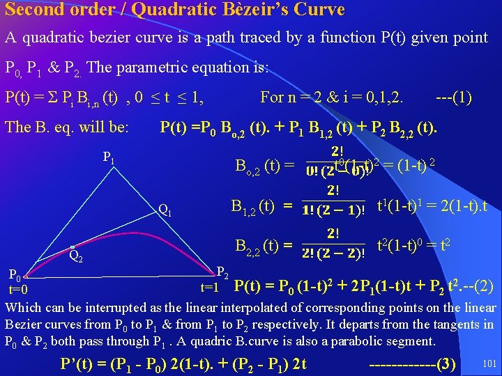
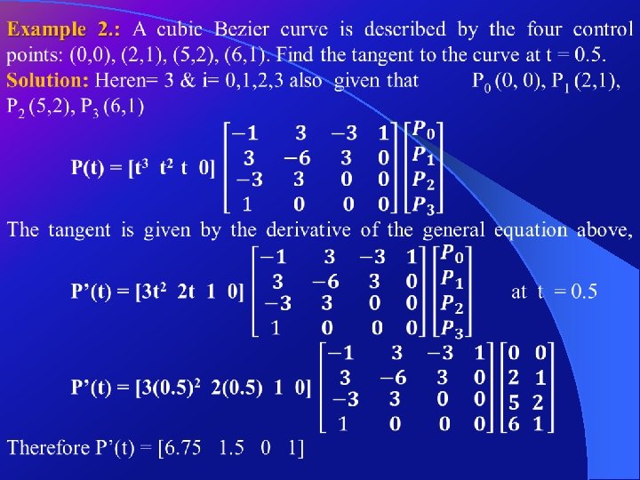
Second order / Quadratic Bèzeir’s Curve A quadratic bezier curve is a path traced by a function P(t) given point P 0, P 1 & P 2. The parametric equation is: P(t) = Σ Pi Bi, n (t) , 0 ≤ t ≤ 1, The B. eq. will be: ---(1) P(t) =P 0 Bo, 2 (t). + P 1 B 1, 2 (t) + P 2 B 2, 2 (t). P 1 Bo, 2 (t) = Q 1 Q 2 For n = 2 & i = 0, 1, 2. t 0(1 -t)2 = (1 -t) 2 B 1, 2 (t) = t 1(1 -t)1 = 2(1 -t). t B 2, 2 (t) = t 2(1 -t)0 = t 2 P 0 t=1 P(t) = P 0 (1 -t)2 + 2 P 1(1 -t)t + P 2 t 2. --(2) t=0 Which can be interrupted as the linear interpolated of corresponding points on the linear Bezier curves from P 0 to P 1 & from P 1 to P 2 respectively. It departs from the tangents in P 0 & P 2 both pass through P 1. A quadric B. curve is also a parabolic segment. P’(t) = (P 1 - P 0) 2(1 -t). + (P 2 - P 1) 2 t ------(3) 101

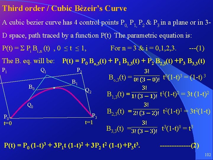
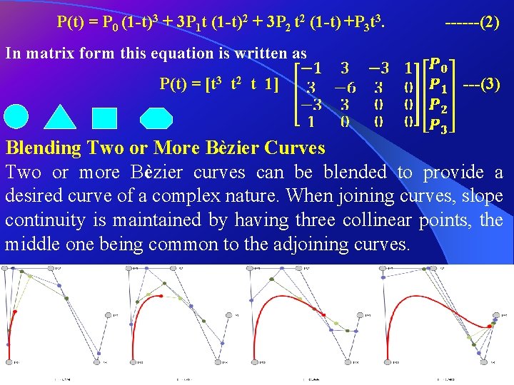
Third order / Cubic Bèzeir’s Curve A cubic bezier curve has 4 control points P 0, P 1, P 2 & P 3 in a plane or in 3 D space, path traced by a function P(t). The parametric equation is: P(t) = Σ Pi Bi, n (t) , 0 ≤ t ≤ 1, The B. eq. will be: P 1 Q 1 B 0 ---(1) P(t) = P 0 Bo, 3(t) + P 1 B 1, 3(t) + P 2 B 2, 3(t) +P 3 B 3, 3(t) P 2 B 1 Q 2 Q 0 P 0 t=0 For n = 3 & i = 0, 1, 2, 3. P 3 t=1 Bo, 3(t) = t 0(1 -t)3 = (1 -t) 3 B 1, 3(t) = t 1(1 -t)2 = 3 t (1 -t)2 B 2, 3(t) = t 2(1 -t)1 = 3 t 2(1 -t) B 3, 3(t) = t 3(1 -t)0 = t 3 P(t) = P 0 (1 -t)3 + 3 P 1 t (1 -t)2 + 3 P 2 t 2 (1 -t) +P 3 t 3. -------(2) 102

P(t) = P 0 (1 -t)3 + 3 P 1 t (1 -t)2 + 3 P 2 t 2 (1 -t) +P 3 t 3. ------(2) In matrix form this equation is written as P(t) = [t 3 t 2 t 1] ---(3) Blending Two or More Bèzier Curves Two or more Bèzier curves can be blended to provide a desired curve of a complex nature. When joining curves, slope continuity is maintained by having three collinear points, the middle one being common to the adjoining curves. 103

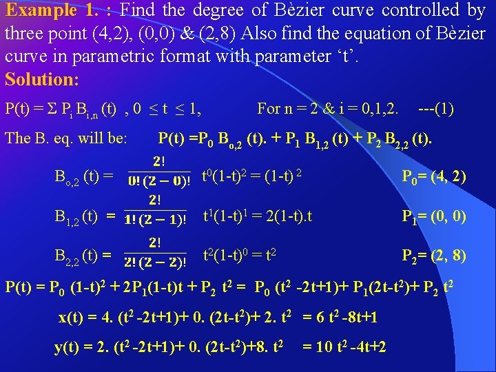
Example 1. : Find the degree of Bèzier curve controlled by three point (4, 2), (0, 0) & (2, 8) Also find the equation of Bèzier curve in parametric format with parameter ‘t’. Solution: P(t) = Σ Pi Bi, n (t) , 0 ≤ t ≤ 1, The B. eq. will be: For n = 2 & i = 0, 1, 2. ---(1) P(t) =P 0 Bo, 2 (t). + P 1 B 1, 2 (t) + P 2 B 2, 2 (t). Bo, 2 (t) = t 0(1 -t)2 = (1 -t) 2 P 0= (4, 2) B 1, 2 (t) = t 1(1 -t)1 = 2(1 -t). t P 1= (0, 0) B 2, 2 (t) = t 2(1 -t)0 = t 2 P 2= (2, 8) P(t) = P 0 (1 -t)2 + 2 P 1(1 -t)t + P 2 t 2 = P 0 (t 2 -2 t+1)+ P 1(2 t-t 2)+ P 2 t 2 x(t) = 4. (t 2 -2 t+1)+ 0. (2 t-t 2)+ 2. t 2 = 6 t 2 -8 t+1 y(t) = 2. (t 2 -2 t+1)+ 0. (2 t-t 2)+8. t 2 = 10 t 2 -4 t+2

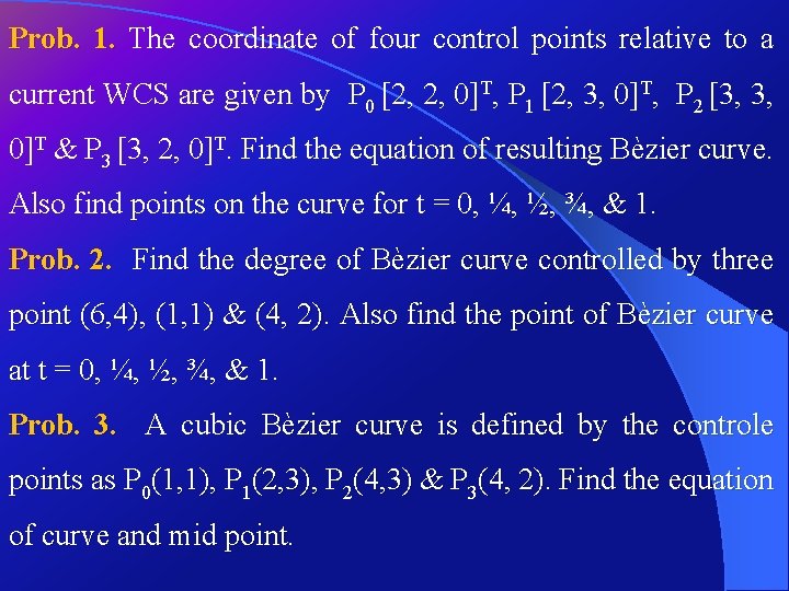
Prob. 1. The coordinate of four control points relative to a current WCS are given by P 0 [2, 2, 0]T, P 1 [2, 3, 0]T, P 2 [3, 3, 0]T & P 3 [3, 2, 0]T. Find the equation of resulting Bèzier curve. Also find points on the curve for t = 0, ¼, ½, ¾, & 1. Prob. 2. Find the degree of Bèzier curve controlled by three point (6, 4), (1, 1) & (4, 2). Also find the point of Bèzier curve at t = 0, ¼, ½, ¾, & 1. Prob. 3. A cubic Bèzier curve is defined by the controle points as P 0(1, 1), P 1(2, 3), P 2(4, 3) & P 3(4, 2). Find the equation of curve and mid point.

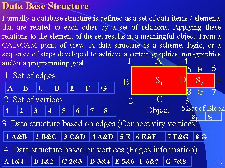
Data Base Structure Formally a database structure is defined as a set of data items / elements that are related to each other by a set of relations. Applying these relations to the element of the set results in a meaningful object. From a CAD/CAM point of view. A data structure is a scheme, logic, or a sequence of steps developed to achieve a certain graphics, non-graphics 1 A 4 and/or a programming goal. 1. Set of edges A B C D E F G 2. Set of vertices 1 2 3 4 5 B 2 6 7 8 S 1 C Object 5 E 6 D S 2 F 8 G 7 3 5. Set of Block S 1 3. Data structure based on edges (Connectivity vertices) 1 -A&B 2 -B&C 3 -C&D 4 -A&D 5 -E 6 -E&F S 2 7 -F&G 8 -G 4. Data structure based on vertices (Edges information) A-1&4 B-1&2 C-2&3 D-3&4 E-5&6 F-6&7 G-7&8 107

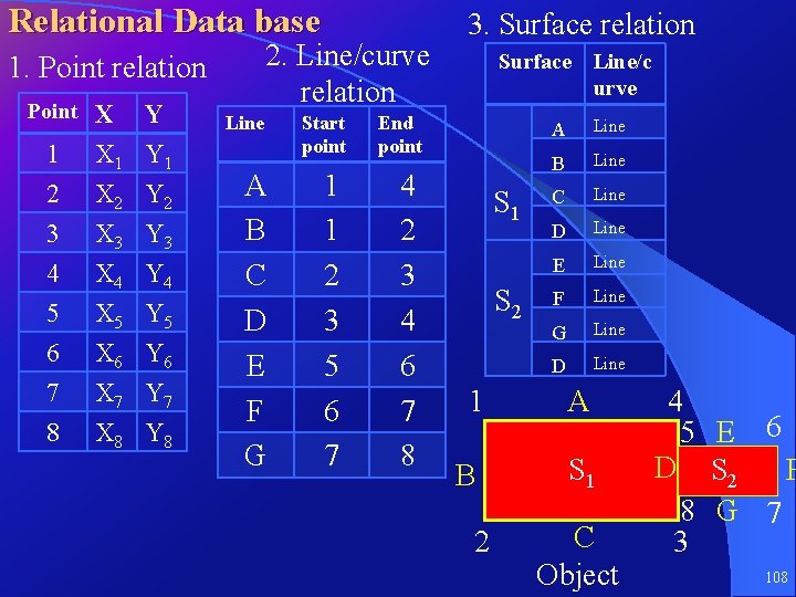
Relational Data base 2. Line/curve relation 1. Point relation Point 1 2 3 X X 1 X 2 X 3 Y Y 1 Y 2 Y 3 4 5 6 X 4 Y 4 X 5 Y 5 X 6 Y 6 7 8 X 7 Y 7 X 8 Y 8 Line A B C D E F G Start point 1 1 2 3 5 6 7 3. Surface relation Surface Line/c urve End point 4 2 3 4 6 7 8 S 1 S 2 A Line B Line C Line D Line E Line F Line G Line D Line 1 A B S 1 2 C Object 4 5 E 6 D S 2 F 8 G 7 3 108

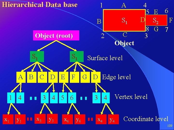
Hierarchical Data base Object (root) S 1 x 1 y 1 S 1 y 3 x 6 B S 1 C Object 4 5 E 6 D S 2 F 8 G 7 3 Surface level G D Edge level 3 4 5 6 x 3 A 2 A B C D E F 1 4 1 3 4 y 6 x 4 Vertex level y 4 Coordinate level 109

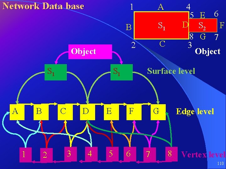
Network Data base 1 A B S 1 A B 1 2 Surface level S 1 C D 3 4 C 2 Object E 5 4 5 E 6 D S 2 F 8 G 7 3 Object F 6 G 7 Edge level 8 Vertex level 110