Treewidth Applications and some Recent Developments Chandra Chekuri

Treewidth, Applications, and some Recent Developments Chandra Chekuri Univ. of Illinois, Urbana-Champaign

Goals of Tutorial • Give an intuitive understanding of treewidth and tree decompositions • Describe some algorithmic applications • Describe some recent developments

Graphs Powerful modeling tool Numerous applications However, many natural problems are intractable Question: • What graph properties allow tractability? • How can they be leveraged in applications?

Graph Properties/Parameters • Sparsity • Connectivity • Topological properties (planarity, genus, . . . ) • Spectral properties (expansion, . . . ) • . . .

Graph Properties/Parameters • Sparsity • Connectivity • Topological properties (planarity, genus, . . . ) • Spectral properties (expansion, . . . ) • . . . • Decomposability

Tree decompositions and Treewidth Studied by [Halin’ 76] Again by [Robertson & Seymour’ 84] as part of their seminal graph minor project In ML tree decompositions related to junction trees

Tree decompositions and Treewidth • key to graph minor theory of Robertson & Seymour • many algorithmic applications Message: algorithms and structural understanding intertwined

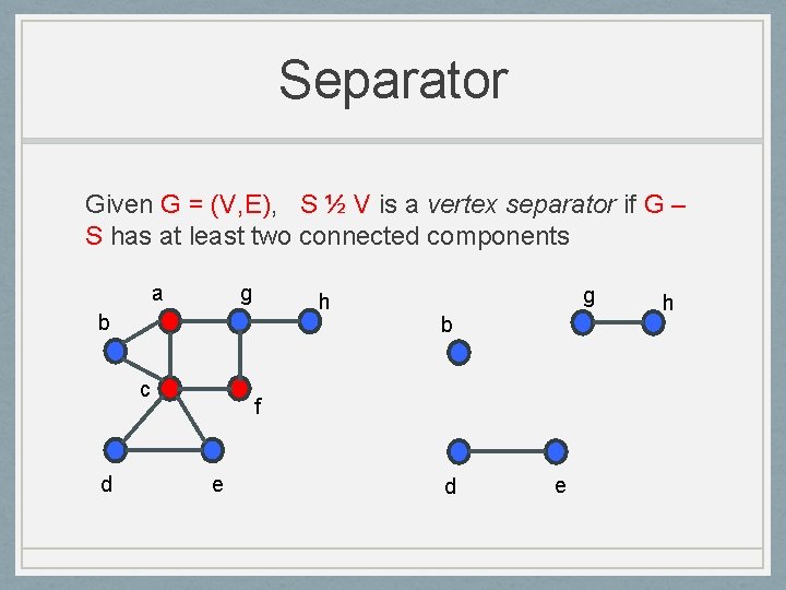
Separator Given G = (V, E), S ½ V is a vertex separator if G – S has at least two connected components a g h b c d g b f e d e h

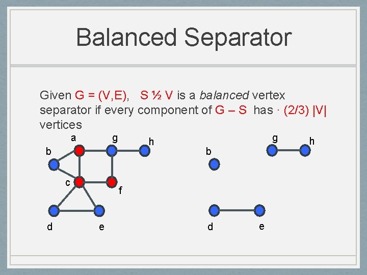
Balanced Separator Given G = (V, E), S ½ V is a balanced vertex separator if every component of G – S has · (2/3) |V| vertices a g h b c d g b f e d e h

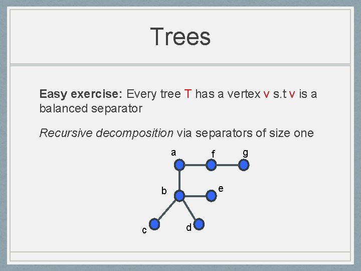
Trees Easy exercise: Every tree T has a vertex v s. t v is a balanced separator Recursive decomposition via separators of size one a e b c g f d

Planar Separator Theorem [Lipton-Tarjan’ 79] Every n vertex planar graph has a balanced separator of size O(√n)

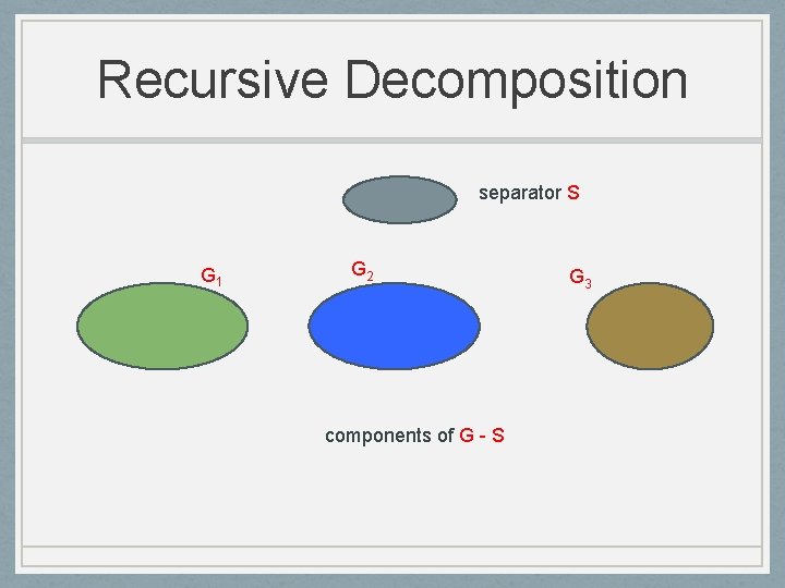
Recursive Decomposition separator S G 1 G 2 components of G - S G 3

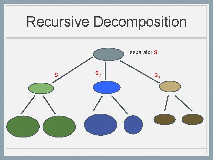
Recursive Decomposition separator S S 1 S 2 S 3

Planar Separator Theorem [Lipton-Tarjan’ 79] Every n vertex planar graph has a balance separator of size O(√n) Many applications via recursive decomposition

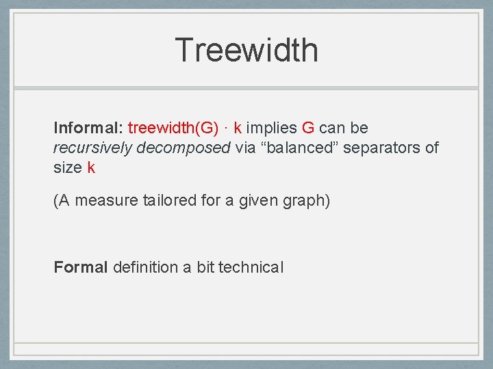
Treewidth Informal: treewidth(G) · k implies G can be recursively decomposed via “balanced” separators of size k (A measure tailored for a given graph) Formal definition a bit technical

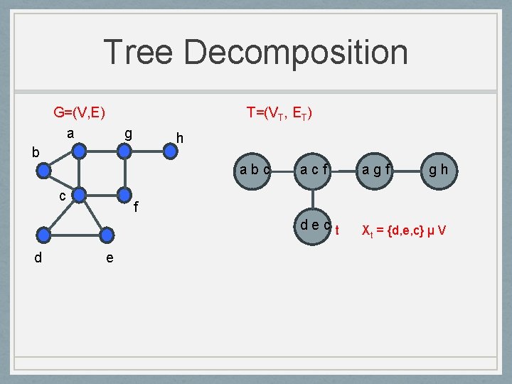
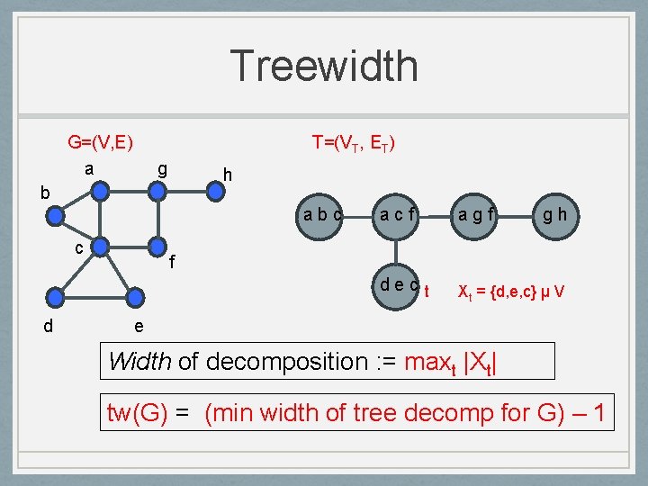
Tree Decomposition G=(V, E) a T=(VT, ET) g h b abc c d acf agf gh dec t Xt = {d, e, c} µ V f e

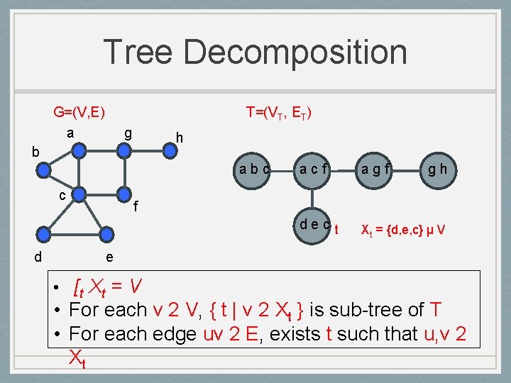
Tree Decomposition G=(V, E) a T=(VT, ET) g h b abc c d acf agf gh dec t Xt = {d, e, c} µ V f e • [t X t = V • For each v 2 V, { t | v 2 Xt } is sub-tree of T • For each edge uv 2 E, exists t such that u, v 2 Xt

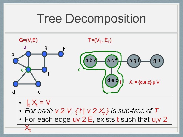
Tree Decomposition G=(V, E) a T=(VT, ET) g h b abc c d f acf agf gh dec t Xt = {d, e, c} µ V c e • [t X t = V • For each v 2 V, { t | v 2 Xt } is sub-tree of T • For each edge uv 2 E, exists t such that u, v 2 Xt

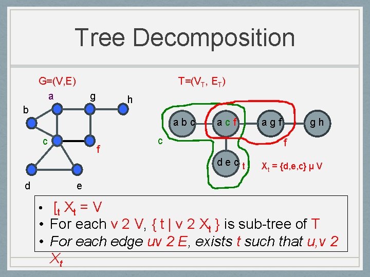
Tree Decomposition G=(V, E) a T=(VT, ET) g h b abc c f acf c gh f dec t d agf Xt = {d, e, c} µ V e • [t X t = V • For each v 2 V, { t | v 2 Xt } is sub-tree of T • For each edge uv 2 E, exists t such that u, v 2 Xt

Treewidth G=(V, E) a T=(VT, ET) g h b abc c d acf agf gh dec t Xt = {d, e, c} µ V f e Width of decomposition : = maxt |Xt| tw(G) = (min width of tree decomp for G) – 1

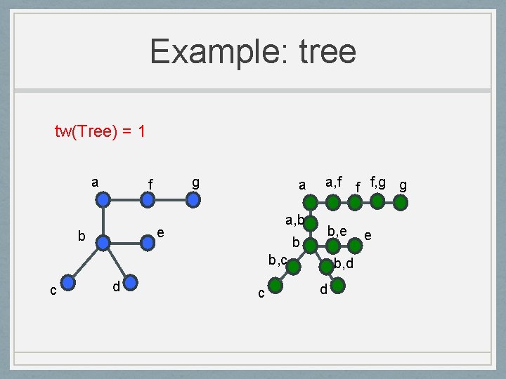
Example: tree tw(Tree) = 1 a g f a a, b e b a, f b, e b b, c c d c b, d d f f, g g e

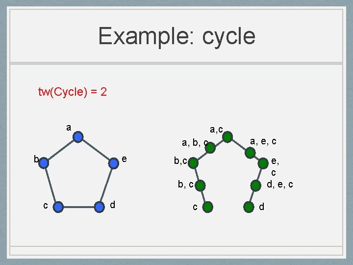
Example: cycle tw(Cycle) = 2 a a, c a, b, c e b a, e, c b, c e, c d, e, c b, c c d

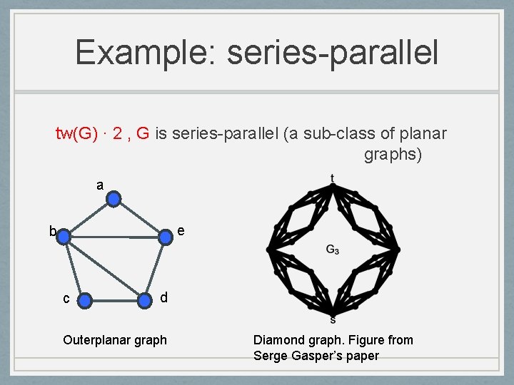
Example: series-parallel tw(G) · 2 , G is series-parallel (a sub-class of planar graphs) a e b c d Outerplanar graph Diamond graph. Figure from Serge Gasper’s paper

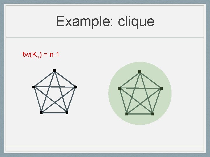
Example: clique tw(Kn) = n-1

Treewidth and separators tw(G) · k implies G can be recursively decomposed via “balanced” separators of size k Approximate converse also holds: If there is a subgraph H of G with no balanced separator of size k then tw(G) ¸ k/c

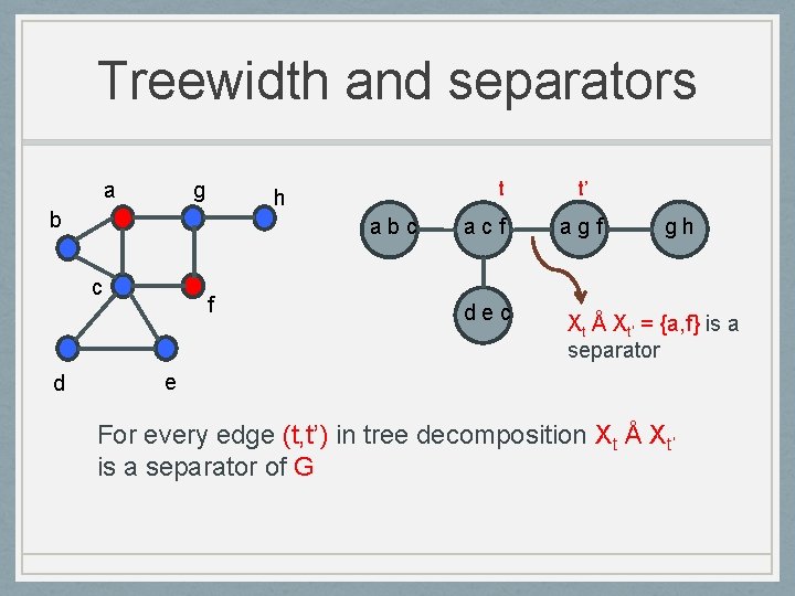
Treewidth and separators a g b abc c d t h f acf dec t’ agf gh Xt Å Xt’ = {a, f} is a separator e For every edge (t, t’) in tree decomposition Xt Å Xt’ is a separator of G

Recursive decomposition tw(G) · k implies G can be recursively decomposed via “balanced” separators of size k • tw(G) · k implies G has a balanced separator S of size k • Recursively decompose graphs in G - S • tw(H) · tw(G) for any subgraph H of G

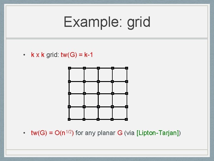
Example: grid • k x k grid: tw(G) = k-1 • tw(G) = O(n 1/2) for any planar G (via [Lipton-Tarjan])

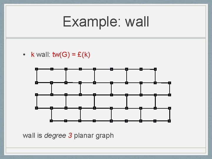
Example: wall • k wall: tw(G) = £(k) wall is degree 3 planar graph

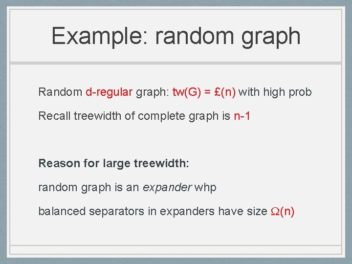
Example: random graph Random d-regular graph: tw(G) = £(n) with high prob Recall treewidth of complete graph is n-1 Reason for large treewidth: random graph is an expander whp balanced separators in expanders have size (n)

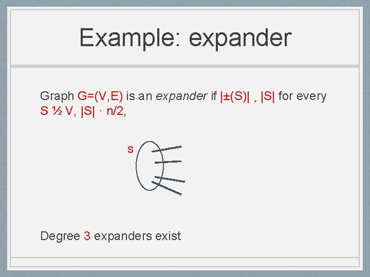
Example: expander Graph G=(V, E) is an expander if |±(S)| ¸ |S| for every S ½ V, |S| · n/2, S Degree 3 expanders exist

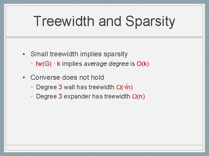
Treewidth and Sparsity • Small treewidth implies sparsity • tw(G) · k implies average degree is O(k) • Converse does not hold • Degree 3 wall has treewidth (√n) • Degree 3 expander has treewidth (n)

Complexity of Treewidth [Arnborg-Corneil-Proskurowski’ 87] Given G, k checking if tw(G) · k is NP-Complete [Bodleander’ 93] 3 O(kk n) time algorithm to check if tw(G) · k (for fixed k, linear time) [Bodleander et al’ 2013] O(ck n) time 5 -approximation

Complexity of Treewidth ®-approx. for node separators implies O(®)-approx. for treewidth [Feige-Hajiaghayi-Lee’ 05] Polynomial time algorithm to output tree decomposition of width · c tw(G) √log tw(G)

Applications of Treewidth • Graph Theory • Polynomial-time algorithms for problems on graphs/structures with bounded/fixed treewidth • Fixed parameter tractability • Approximation algorithms

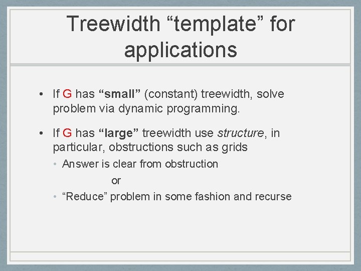
Treewidth “template” for applications • If G has “small” (constant) treewidth, solve problem via dynamic programming. • If G has “large” treewidth use structure, in particular, obstructions such as grids • Answer is clear from obstruction or • “Reduce” problem in some fashion and recurse

Outline • Topic I: Leveraging small treewidth • dynamic programming based algorithms • reducing to small treewidth • Topic II: Interplay of small and large treewidth • fixed parameter intractability • Topic III: Large treewidth for approximation • disjoint paths and recent developments on structure

Algorithms for bounded/small treewidth graphs Dynamic programming based algorithms for trees extends naturally to bounded treewidth graphs Consequence: Many hard problems can be solved efficiently in graphs of small treewidth

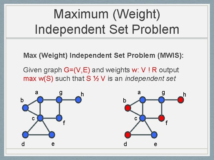
Maximum (Weight) Independent Set Problem Max (Weight) Independent Set Problem (MWIS): Given graph G=(V, E) and weights w: V ! R output max w(S) such that S ½ V is an independent set a g h b c d a h b c f e g d f e

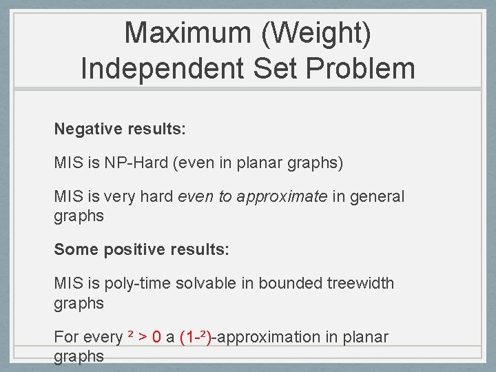
Maximum (Weight) Independent Set Problem Negative results: MIS is NP-Hard (even in planar graphs) MIS is very hard even to approximate in general graphs Some positive results: MIS is poly-time solvable in bounded treewidth graphs For every ² > 0 a (1 -²)-approximation in planar graphs

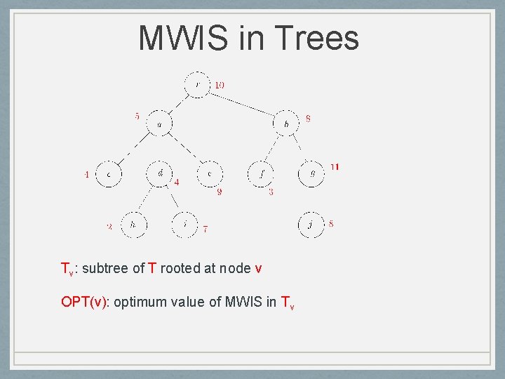
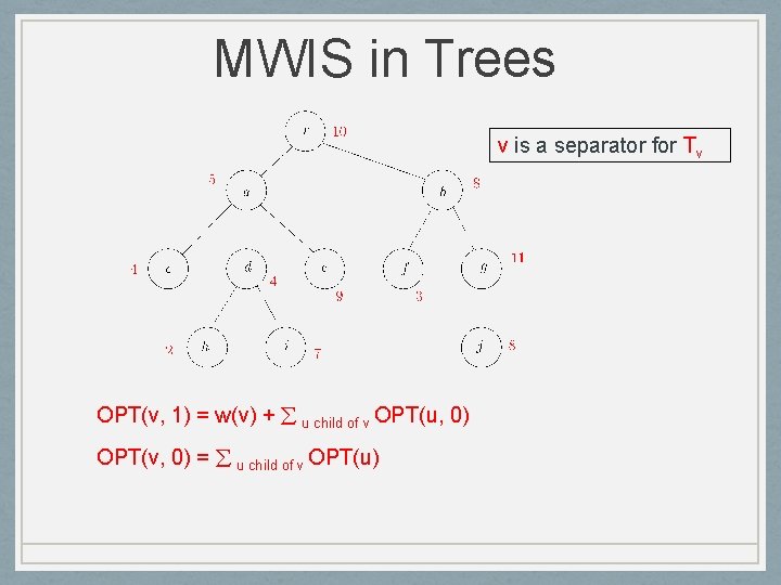
MWIS in Trees Tv: subtree of T rooted at node v OPT(v): optimum value of MWIS in Tv

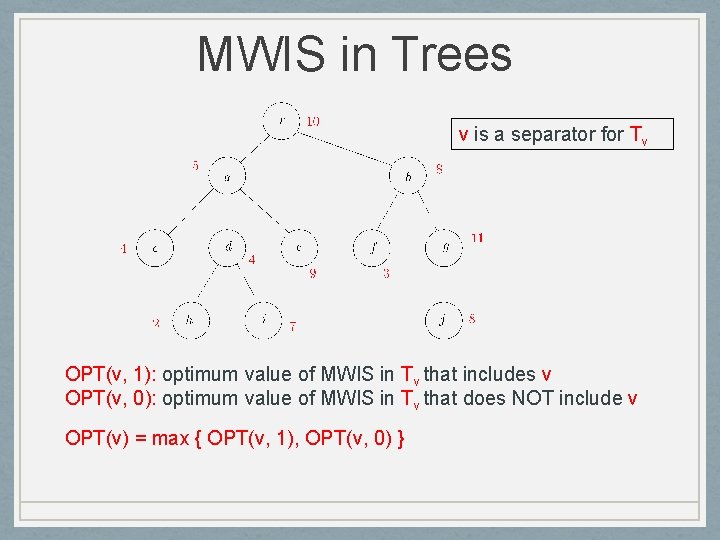
MWIS in Trees v is a separator for Tv OPT(v, 1): optimum value of MWIS in Tv that includes v OPT(v, 0): optimum value of MWIS in Tv that does NOT include v OPT(v) = max { OPT(v, 1), OPT(v, 0) }

MWIS in Trees v is a separator for Tv OPT(v, 1) = w(v) + u child of v OPT(u, 0) OPT(v, 0) = u child of v OPT(u)

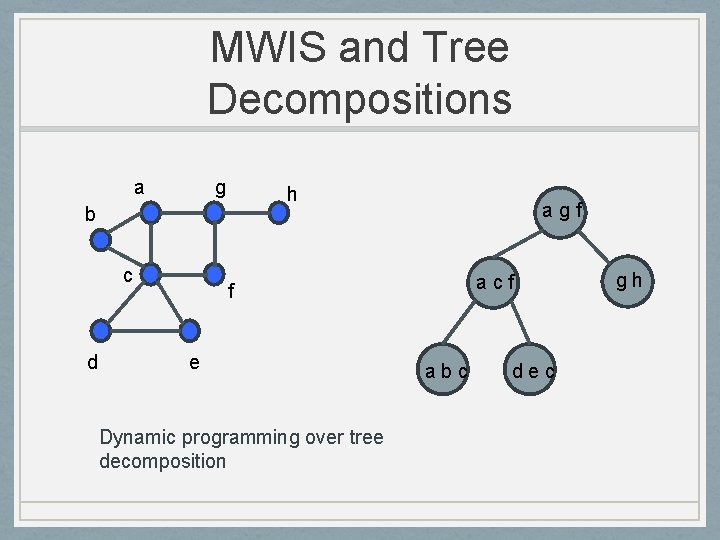
MWIS and Tree Decompositions a g h b c d agf acf f e Dynamic programming over tree decomposition abc dec gh

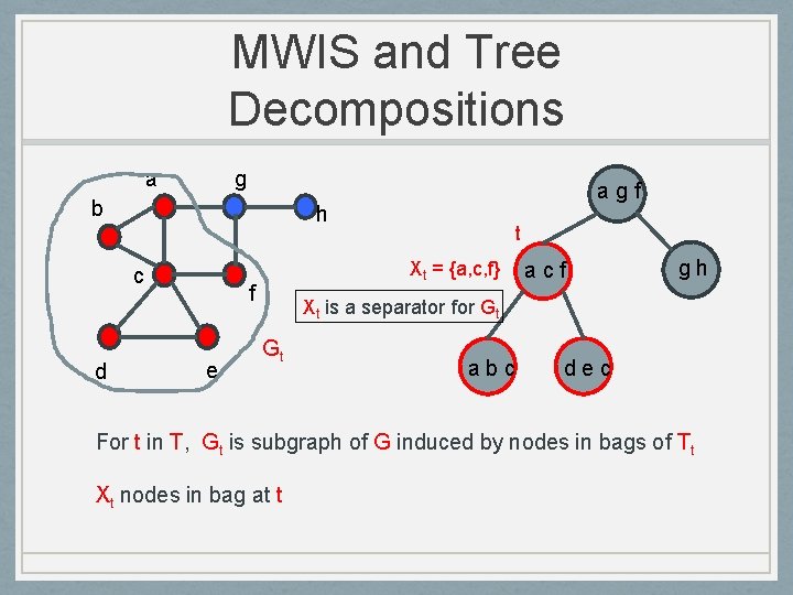
MWIS and Tree Decompositions a g b h c d agf Xt = {a, c, f} f e t acf gh Xt is a separator for Gt Gt abc dec For t in T, Gt is subgraph of G induced by nodes in bags of Tt Xt nodes in bag at t

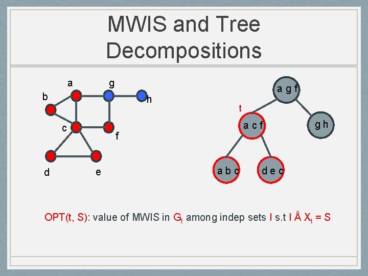
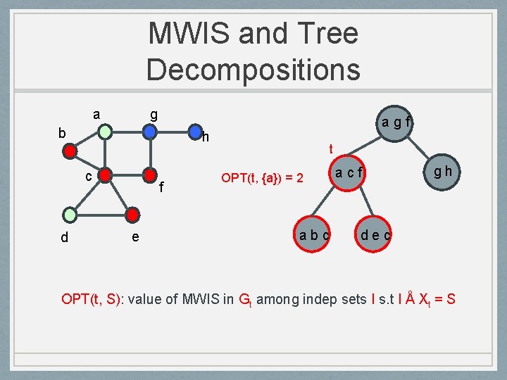
MWIS and Tree Decompositions a g b h c d agf t acf f e abc gh dec OPT(t, S): value of MWIS in Gt among indep sets I s. t I Å Xt = S

MWIS and Tree Decompositions a g b h c d agf f e t OPT(t, {a}) = 2 abc acf gh dec OPT(t, S): value of MWIS in Gt among indep sets I s. t I Å Xt = S

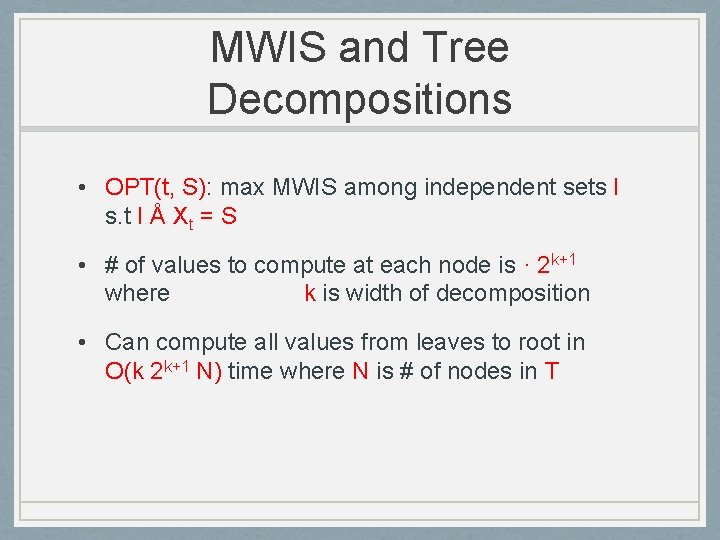
MWIS and Tree Decompositions • OPT(t, S): max MWIS among independent sets I s. t I Å Xt = S • # of values to compute at each node is · 2 k+1 where k is width of decomposition • Can compute all values from leaves to root in O(k 2 k+1 N) time where N is # of nodes in T

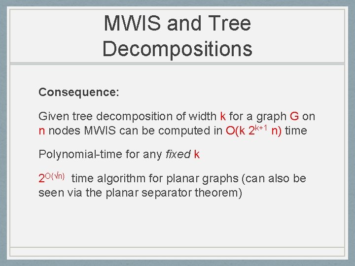
MWIS and Tree Decompositions Consequence: Given tree decomposition of width k for a graph G on n nodes MWIS can be computed in O(k 2 k+1 n) time Polynomial-time for any fixed k 2 O(√n) time algorithm for planar graphs (can also be seen via the planar separator theorem)

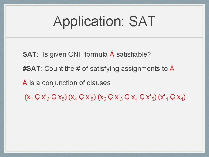
Application: SAT: Is given CNF formula Á satisfiable? #SAT: Count the # of satisfying assignments to Á Á is a conjunction of clauses (x 1 Ç x’ 3 Ç x 5) (x 4 Ç x’ 5) (x 2 Ç x’ 3 Ç x 4 Ç x’ 5) (x’ 1 Ç x 4)

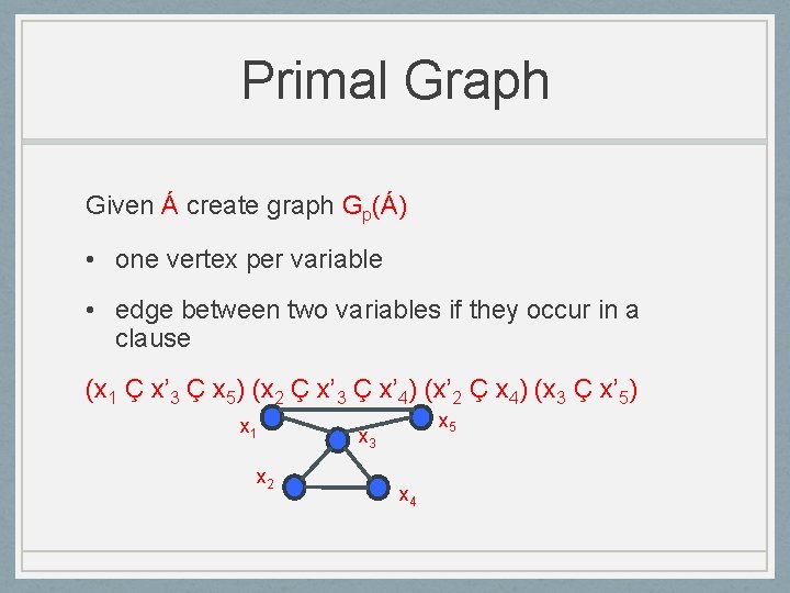
Primal Graph Given Á create graph Gp(Á) • one vertex per variable • edge between two variables if they occur in a clause (x 1 Ç x’ 3 Ç x 5) (x 2 Ç x’ 3 Ç x’ 4) (x’ 2 Ç x 4) (x 3 Ç x’ 5) x 1 x 2 x 5 x 3 x 4

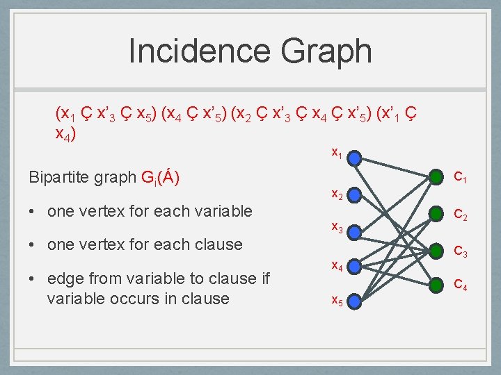
Incidence Graph (x 1 Ç x’ 3 Ç x 5) (x 4 Ç x’ 5) (x 2 Ç x’ 3 Ç x 4 Ç x’ 5) (x’ 1 Ç x 4) x 1 Bipartite graph Gi(Á) • one vertex for each variable C 1 x 2 x 3 • one vertex for each clause • edge from variable to clause if variable occurs in clause x 4 x 5 C 2 C 3 C 4

SAT O(ck size(Á)) time algorithm for SAT and #SAT where k = tw(Gp(Á)) or k = tw(Gi(Á)) Question: which graph is better to use?

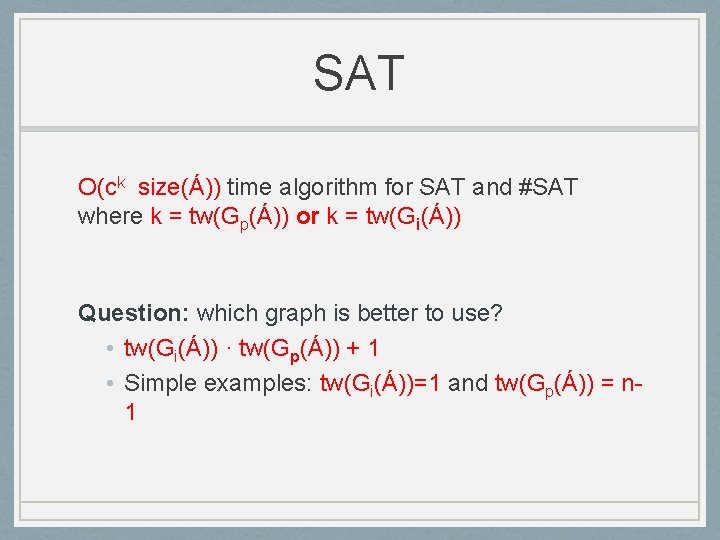
SAT O(ck size(Á)) time algorithm for SAT and #SAT where k = tw(Gp(Á)) or k = tw(Gi(Á)) Question: which graph is better to use? • tw(Gi(Á)) · tw(Gp(Á)) + 1 • Simple examples: tw(Gi(Á))=1 and tw(Gp(Á)) = n 1

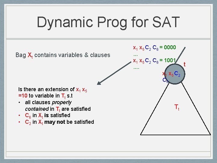
Dynamic Prog for SAT Bag Xt contains variables & clauses Is there an extension of x 1 x 5 =10 to variable in Tt s. t • all clauses properly contained in Tt are satisfied • C 6 in Xt is satisfied • C 2 in Xt may not be satisfied x 1 x 5 C 2 C 6 = 0000. . . x 1 x 5 C 2 C 6 = 1001 t. . x 1 x 5 C 2 C 6 Tt

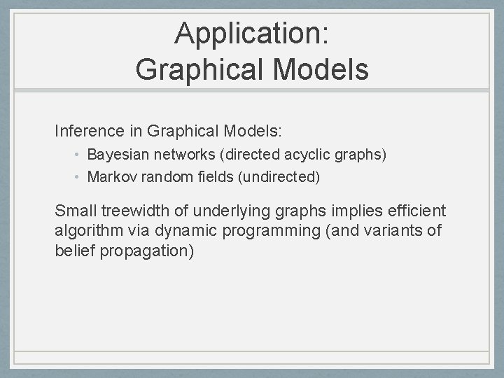
Application: Graphical Models Inference in Graphical Models: • Bayesian networks (directed acyclic graphs) • Markov random fields (undirected) Small treewidth of underlying graphs implies efficient algorithm via dynamic programming (and variants of belief propagation)

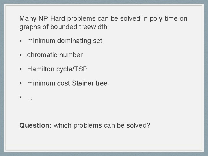
Many NP-Hard problems can be solved in poly-time on graphs of bounded treewidth • minimum dominating set • chromatic number • Hamilton cycle/TSP • minimum cost Steiner tree • . . . Question: which problems can be solved?

Courcelle’s Theorem A meta-algorithmic result via logic: [Courcelle’ 90] Any property Á of graphs expressible in EMSO 2 logic can be checked in time f(|Á|, k) n on an n node graph G given a tree decomposition of width k for G. Here f is some computable function. Various extensions of above for optimization/counting and related problems.

Summary Graph/Structure has small/bounded treewidth implies efficient/poly-time algorithm for many intractable problems Next: leveraging bounded treewidth graphs for more general graphs

MWIS in Planar Graphs MWIS is exactly solvable in bounded treewidth graphs Can we extend ideas to broader class of graphs?

Approximation Algorithm Approximation algorithm for optimization problem ¦ • a worst-case polynomial time algorithm • gives a worst-case guarantee on the output of solution • • A(I) – value of solution output by A on instance I OPT(I) – value of an optimum solution for I For maximization: A(I) ¸ ® OPT(I) for all I ® – the approximation ratio of A

MWIS in Planar Graphs [Baker’ 94] There is a polynomial-time approximation scheme (PTAS) for MWIS in planar graphs. Given ² > 0, • Algorithm runs in 2 O(1/²) poly(n) time • Gives a (1 -²) approximation to MWIS

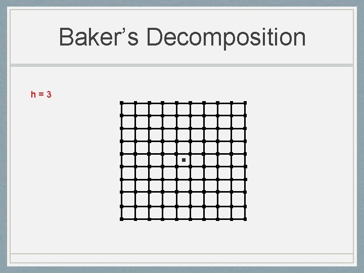
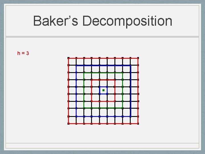
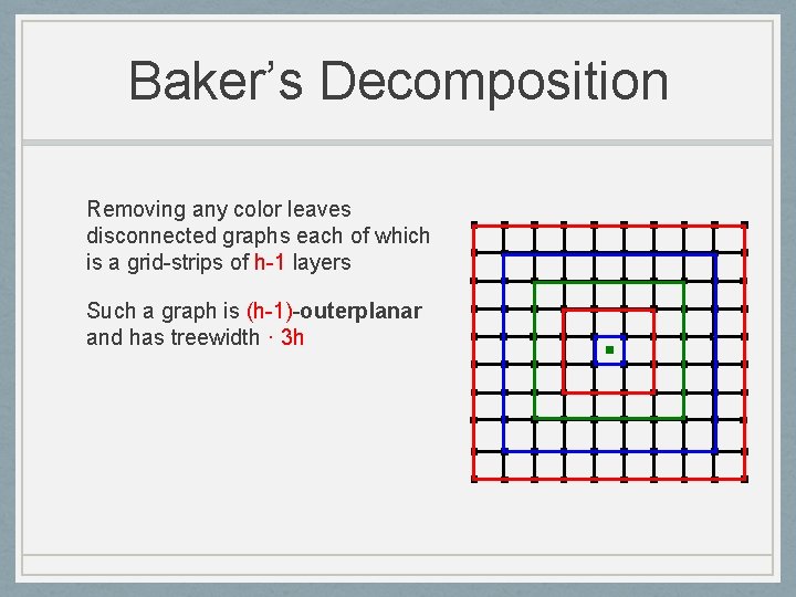
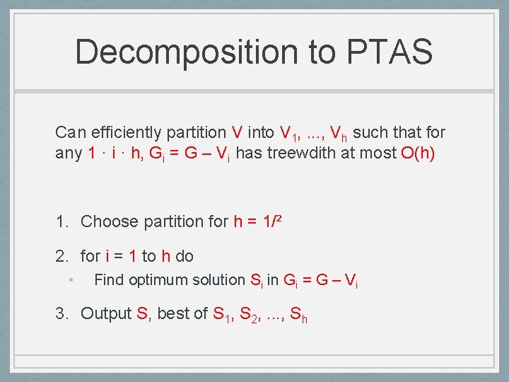
Decomposing Planar Graphs [Baker’ 94] G=(V, E) planar graph, h any non-negative integer Can efficiently partition V into V 1, . . . , Vh such that for any 1 · i · h • Gi = G – Vi has treewdith at most O(h)

Baker’s Decomposition h=3

Baker’s Decomposition h=3

Baker’s Decomposition Removing any color leaves disconnected graphs each of which is a grid-strips of h-1 layers Such a graph is (h-1)-outerplanar and has treewidth · 3 h

Decomposition to PTAS Can efficiently partition V into V 1, . . . , Vh such that for any 1 · i · h, Gi = G – Vi has treewdith at most O(h) 1. Choose partition for h = 1/² 2. for i = 1 to h do • Find optimum solution Si in Gi = G – Vi 3. Output S, best of S 1, S 2, . . . , Sh

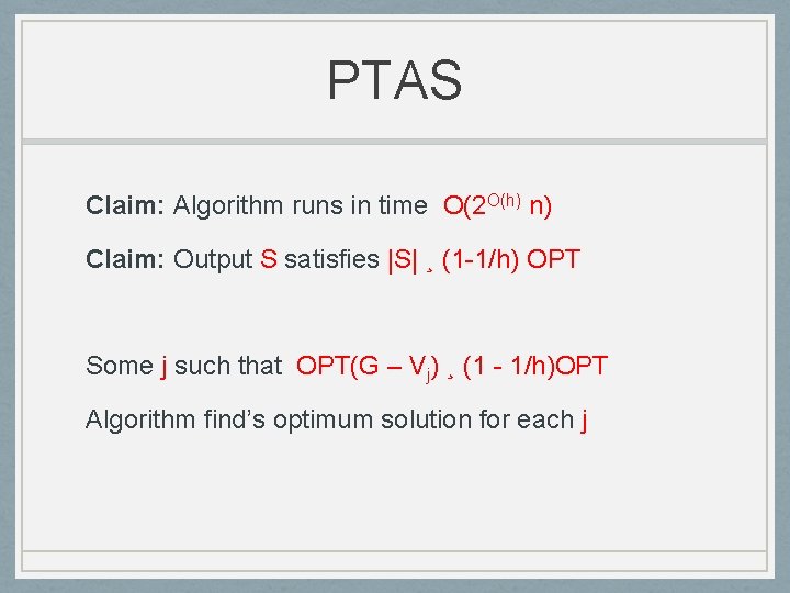
PTAS Claim: Algorithm runs in time O(2 O(h) n) Claim: Output S satisfies |S| ¸ (1 -1/h) OPT Some j such that OPT(G – Vj) ¸ (1 - 1/h)OPT Algorithm find’s optimum solution for each j

Power of Baker: PTASes Galore Baker’s ideas and techniques have been generalized and extended to obtain PTASes: • for H-minor free graphs for any fixed H substantially generalizing results for planar graphs • graphs of bounded “local treewidth” • large number of optimization problems

Summary Bounded treewidth results can be leveraged to provide algorithms/heuristics for much larger and useful classes of graphs

Outline • Topic I: Leveraging small treewidth • dynamic programming based algorithms • reducing to small treewidth • Topic II: Interplay of small and large treewidth • fixed parameter intractability • Topic III: Large treewidth for approximation • disjoint paths and recent developments on structure

Small to Large Treewidth Important applications require a fine/deep understanding of structure of large treewidth graphs Robertson-Seymour theory provides many powerful tools

Fixed Parameter Tractability

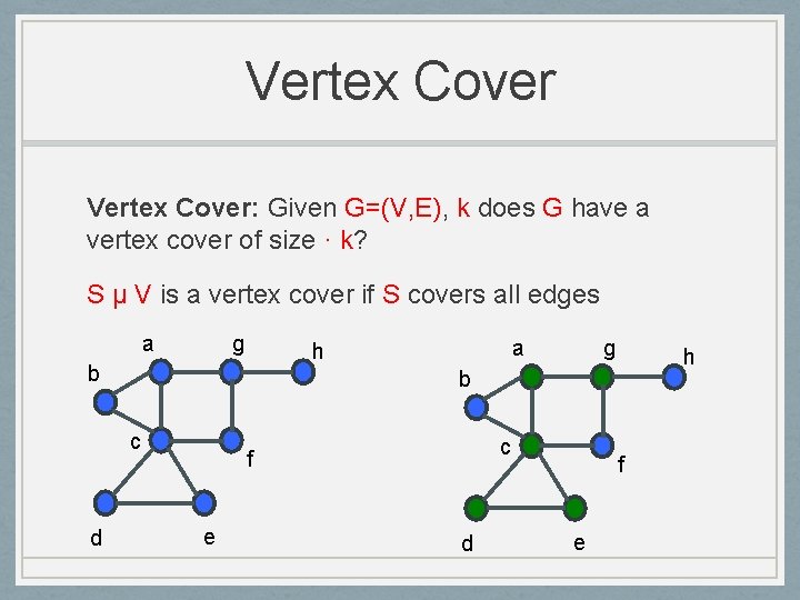
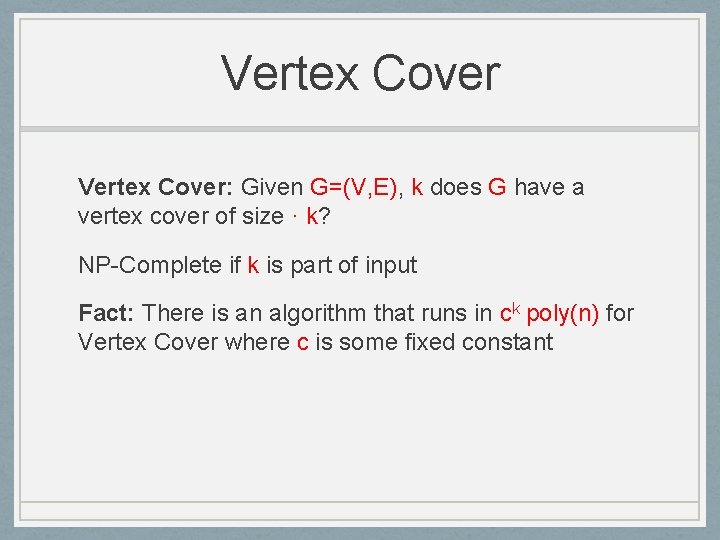
Vertex Cover: Given G=(V, E), k does G have a vertex cover of size · k? S µ V is a vertex cover if S covers all edges a g b g h b c d a h c f e d f e

Vertex Cover: Given G=(V, E), k does G have a vertex cover of size · k? NP-Complete if k is part of input Fact: There is an algorithm that runs in ck poly(n) for Vertex Cover where c is some fixed constant

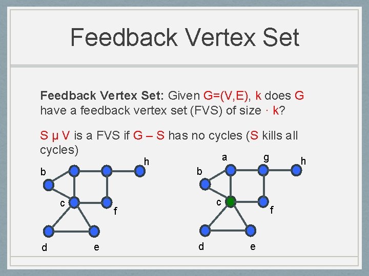
Feedback Vertex Set: Given G=(V, E), k does G have a feedback vertex set (FVS) of size · k? S µ V is a FVS if G – S has no cycles (S kills all cycles) h b c d a b c f e g d f e h

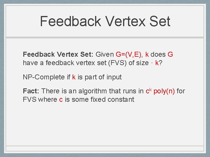
Feedback Vertex Set: Given G=(V, E), k does G have a feedback vertex set (FVS) of size · k? NP-Complete if k is part of input Fact: There is an algorithm that runs in ck poly(n) for FVS where c is some fixed constant

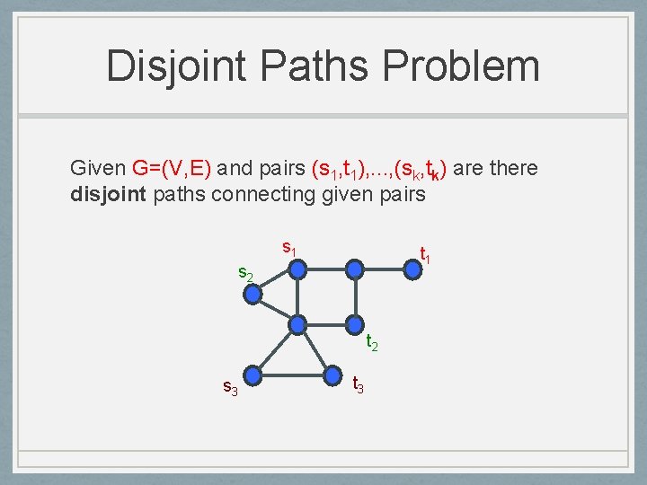
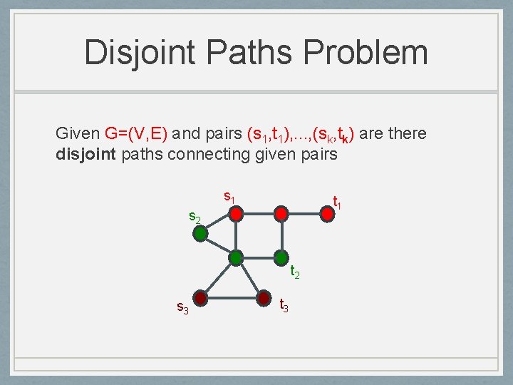
Disjoint Paths Problem Given G=(V, E) and pairs (s 1, t 1), . . . , (sk, tk) are there disjoint paths connecting given pairs s 1 t 1 s 2 t 2 s 3 t 3

Disjoint Paths Problem Given G=(V, E) and pairs (s 1, t 1), . . . , (sk, tk) are there disjoint paths connecting given pairs s 1 t 1 s 2 t 2 s 3 t 3

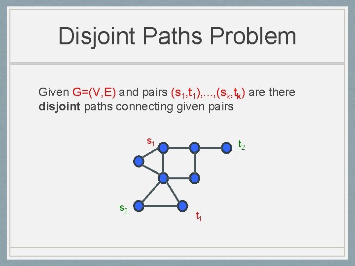
Disjoint Paths Problem Given G=(V, E) and pairs (s 1, t 1), . . . , (sk, tk) are there disjoint paths connecting given pairs s 1 s 2 t 1

Disjoint Paths Problem Given G=(V, E) and pairs (s 1, t 1), . . . , (sk, tk) are there disjoint paths connecting given pairs k = 1 Is there a path from s to t? Easy k = 2 NP-Complete in directed graphs! [FHW’ 80] NP-Complete if k is part of input in undir graphs [Robertson-Seymour] Poly-time solvable for any fixed k in O(n 3) time in undirected graphs

Fixed Parameter Tractability Fixed Parameter Tractable: has algorithm with runtime f(k) poly(n) where k is parameter size and n is instance size • Many different parameterizations possible for a problem • Choice depends on application

FPT and Treewidth Several FPT algorithms can be obtained via treewidth Generic paradigm: 1. If tw(G) is small use exact algorithm via dynamic programming 2. If tw(G) is large use “structure” of G

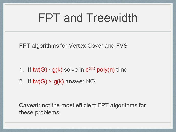
FPT and Treewidth FPT algorithms for Vertex Cover and FVS 1. If tw(G) · g(k) solve in cg(k) poly(n) time 2. If tw(G) > g(k) answer NO Caveat: not the most efficient FPT algorithms for these problems

FPT and Treewidth FPT algorithms for Vertex Cover and FVS 1. If tw(G) · g(k) solve in cg(k) poly(n) time 2. If tw(G) > g(k) answer NO Need to show correctness

Structure of graphs with “large” treewidth What can we say about a graph with “large” treewidth?

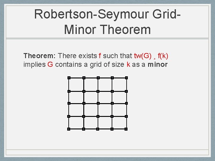
Robertson-Seymour Grid. Minor Theorem: There exists f such that tw(G) ¸ f(k) implies G contains a grid of size k as a minor

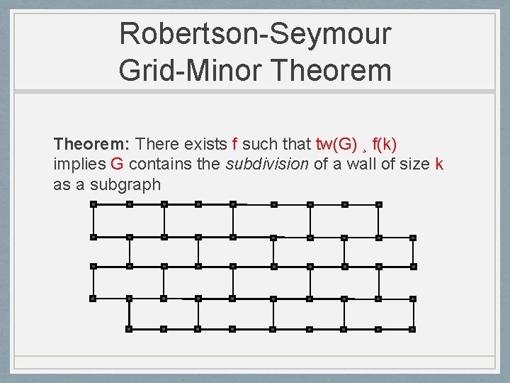
Robertson-Seymour Grid-Minor Theorem: There exists f such that tw(G) ¸ f(k) implies G contains the subdivision of a wall of size k as a subgraph

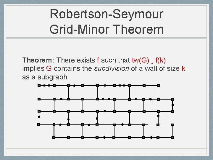
Robertson-Seymour Grid-Minor Theorem: There exists f such that tw(G) ¸ f(k) implies G contains the subdivision of a wall of size k as a subgraph

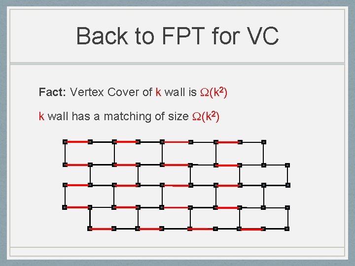
Back to FPT for VC Fact: Vertex Cover of k wall is (k 2) k wall has a matching of size (k 2)

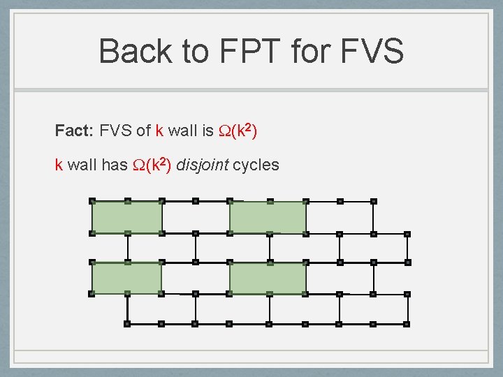
Back to FPT for FVS Fact: FVS of k wall is (k 2) k wall has (k 2) disjoint cycles

FPT and Treewidth FPT algorithms for Vertex Cover and FVS 1. If tw(G) · g(k) solve in cg(k) poly(n) time 2. If tw(G) > g(k) answer NO g(k) = f(c√k) for appropriate constant c suffices

RS Disjoint Path Algorithm 1. If tw(G) · f(k) use dynamic programming 2. Else • • • G has “large” treewidth. Use heavy machinery of graph minor structure theory to find in polynomial time an “irrelevant vertex” v Pairs routable in G iff they are routable in G – v Recurse on G - v

RS Disjoint Paths Algorithm 1. If tw(G) · f(k) use dynamic programming 2. Else • • • G has “large” treewidth. Use heavy machinery of graph minor structure theory to find in polynomial time an “irrelevant vertex” v Pairs routable in G iff they are routable in G – v Recurse on G – v Algorithm/proof requires full power of graph minor machinery. No other algorithmic approach known yet

Summary Important applications require a fine/deep understanding of structure of large treewidth graphs Robertson-Seymour theory provides many powerful tools Quantitative bounds are weak, proofs are hard & long Substantial (ongoing) work on improving bounds, simplifying proofs, and algorithmic applications

Outline • Topic I: Leveraging small treewidth • dynamic programming based algorithms • reducing to small treewidth • Topic II: Interplay of small and large treewidth • fixed parameter intractability • Topic III: Large treewidth for approximation • disjoint paths and recent developments on structure

Robertson-Seymour Grid. Minor Theorem: There exists f such that tw(G) ¸ f(k) implies G contains as a minor a grid of size k

Bounds for Grid Minor Theorem [Robertson-Seymour]: f is “enormous” [Robertson-Seymour-Thomas]: f(k) · 2 c k 5 [Leaf-Seymour, Kawarabayashi-Kobayashi’ 12]: f(k) · 2 c k 2 log k [Robertson-Seymour-Thomas]: If G is planar f(k) · 6 k

Recent Improvement [C-Chuzhoy’ 13] Theorem: tw(G) ¸ k 98+o(1) implies that G has a gridminor of size k x k. Also a poly-time algorithm. First polynomial relationship between treewidth and grid-minor size

Recent Improvement [C-Chuzhoy’ 13] Theorem: tw(G) ¸ k 98+o(1) implies that G has a gridminor of size k x k. Also a poly-time algorithm. Previously: tw(G) = h implies grid of size < √log h Now: tw(G) = h implies grid of size h 1/98 Limit: tw(G) = h cannot get grid of size > √(h/log h)

Other Results on Structure of Large Treewidth Graphs [C-Chuzhoy] • Large routing structures in large treewidth graphs • applications to approximating disjoint paths problems • Treewidth decomposition theorems • applications to fixed parameter tractability • applications to Erdos-Posa type theorems • Treewidth sparsification

Improvements • parameters in various applications improve from “exponential” to “polynomial” (in some cases to near linear) • hardness results conditional on poly-sized gridminor are now “unconditional” • several technical tools of potential future use

Treewidth and Routing Disjoint paths problem: Given G=(V, E) and pairs (s 1, t 1), . . . , (sk, tk) are there disjoint paths connecting given pairs Optimization version: maximize # of pairs routed NP-Hard when k is part of input even on trees Can we approximate well?

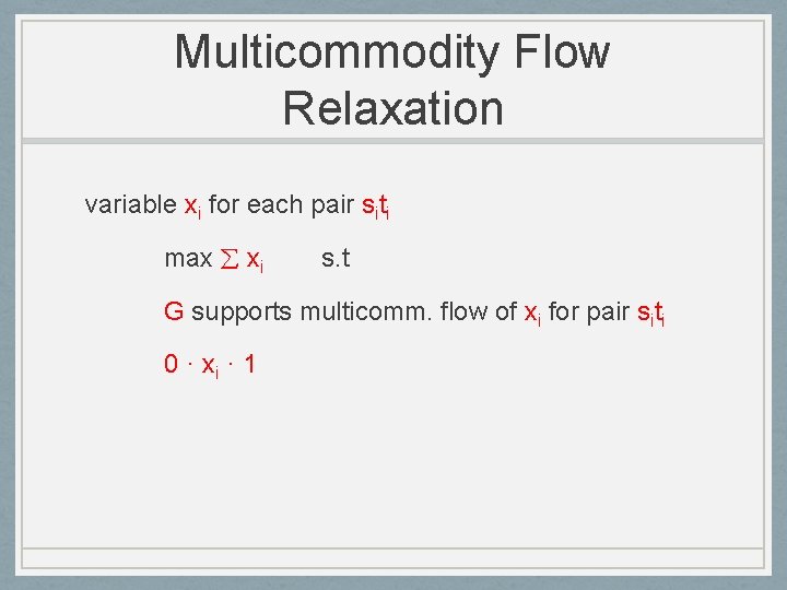
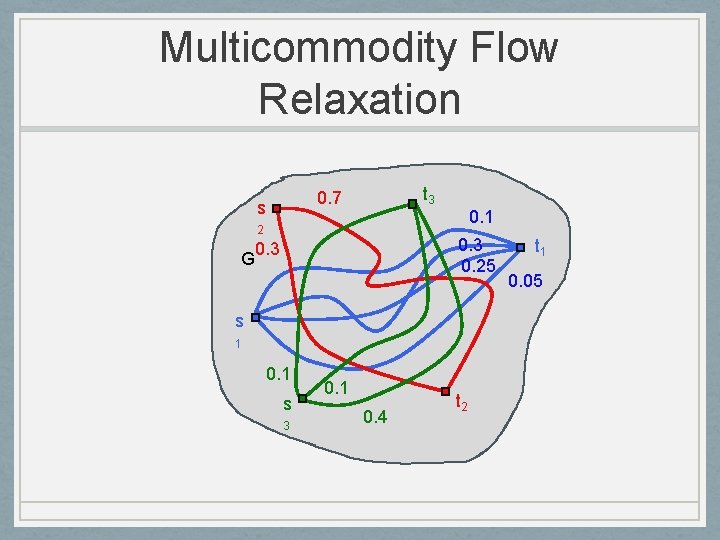
Multicommodity Flow Relaxation variable xi for each pair siti max xi s. t G supports multicomm. flow of xi for pair siti 0 · xi · 1

Multicommodity Flow Relaxation t 3 0. 7 s 2 G 0. 1 0. 3 0. 25 0. 3 s 1 0. 1 s 3 0. 1 0. 4 t 2 t 1 0. 05

Integrality Gap tk tk-1 ti t 3 t 2 [GVY] (n 1/2) gap t 1 sk sk-1 si s 3 s 2 s 1

Routing with Congestion Can we route many pairs if we allow 2 paths per node? Can we route many pairs if capacity of each node is 2? “many pairs” compared to OPTLP the value of flow

Routing with Congestion Can we route many pairs if we allow 2 paths per node? Can we route many pairs if capacity of each node is 2? Question finally resolved in the affirmative!

Reduction to Treewidth Question [C-Khanna-Shepherd’ 05] If treewidth(G) = k does G have a “routing structure” of size comparable to k? In particular (k/polylog(k)) ?

Treewidth and Routing Question: If tw(G) = k does G have a large routing structure? [Robertson-Seymour-Thomas] If tw(G) = k and G is planar then G has a grid-minor of size (k) Grid minors are good routing structures.

[C-Khanna-Shepherd’ 05] Route many pairs to the grid

[C-Khanna-Shepherd’ 05] Route many pairs to the grid Use grid as a “switch” to connect the pairs with one crossing (congestion 2)

Treewidth and Routing [Rao-Zhou’ 08] Idea for general graphs: “Embed” an expander using cut-matching game of [Khandekar-Rao-Vazirani’ 05]

Treewidth and Routing [Chuzhoy’ 11, Chuzhoy-Li’ 12] If tw(G) ¸ k then there is an expander of size k/polylog(k) that can be “embedded” into G with edge congestion 2 [C-Ene’ 13] If tw(G) ¸ k then there is an expander of size k/polylog(k) that can be “embedded” into G with node congestion 51 [C-Chuzhoy’ 14] improve node congestion to 2

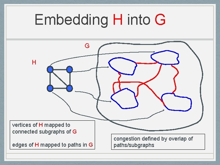
Embedding H into G G H vertices of H mapped to connected subgraphs of G edges of H mapped to paths in G congestion defined by overlap of paths/subgraphs

Treewidth and Routing Bottom line: • can route OPTLP/polylog(k) pairs • congestion 2 • polynomial-time algorithm Resolves a long standing open problem by understanding the structure of “large” treewidth graphs

Treewidth and Routing • Routing work motivated graph theoretic question • Needed very good quantitative parameters in some sense (size of routing structure vs treewidth) • But could relax requirements in another sense (congestion) • Led to several other improvements including the grid-minor theorem

One Last Application

SAT SAT: a fundamental problem in theory and practice Canonical hard problem in theory SAT Solvers: can solve many extremely large instances Explanation?

Easy Cases of SAT Several easy cases of SAT • From Schaefer’s dichotomy theorem (2 -SAT, Horn -SAT. . . ) • Bounded treewidth instances Can a SAT instance be “reduced” to a known easy class?

Backdoors to SAT [Williams-Gomes-Selman’ 03] A SAT formula Á has a “backdoor” if it has a “small” set of variables that make it easy to solve Strong backdoor: S is a strong backdoor if for every assignment a to S the formula ÁS Ã a is easy ÁS Ã a obtained by assigning a to S in Á and simplifying

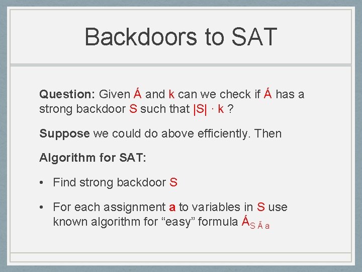
Backdoors to SAT Question: Given Á and k can we check if Á has a strong backdoor S such that |S| · k ?

Backdoors to SAT Question: Given Á and k can we check if Á has a strong backdoor S such that |S| · k ? Suppose we could do above efficiently. Then Algorithm for SAT: • Find strong backdoor S • For each assignment a to variables in S use known algorithm for “easy” formula ÁS Ã a

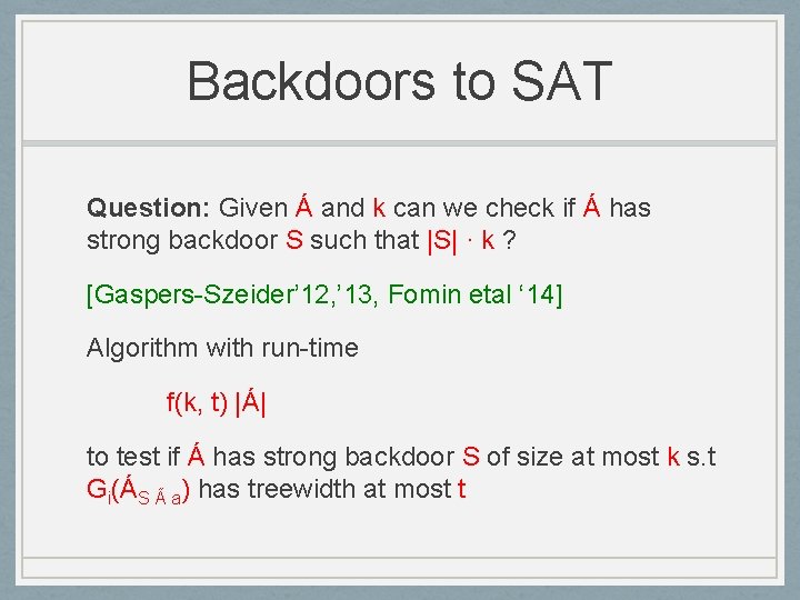
Backdoors to SAT Question: Given Á and k can we check if Á has strong backdoor S such that |S| · k ? [Gaspers-Szeider’ 12, ’ 13, Fomin etal ‘ 14] Algorithm with run-time f(k, t) |Á| to test if Á has strong backdoor S of size at most k s. t Gi(ÁS Ã a) has treewidth at most t

Conclusion • Treewidth & tree decomposition are a powerful way to understand graphs and related structures • Closely connected to separators and recursive decomposability • Many theoretical and conceptual applications • Some practical successes • Hope for more in the future

Thank You!