COMP 4211 Advanced Computer Architectures Algorithms University of



- Slides: 134

COMP 4211 – Advanced Computer Architectures & Algorithms University of NSW Seminar Presentation Semester 2 2004 Software Approaches to Exploiting Instruction Level Parallelism Lecture notes by: David A. Patterson Boris Savkovic

Outline 1. Introduction 2. Basic Pipeline Scheduling 3. Instruction Level Parallelism and Dependencies 4. Local Optimizations and Loops 5. Global Scheduling Approaches 6. HW Support for Aggressive Optimization Strategies TALK TALK

INTRODUCTION How does software based scheduling differ from hardware based scheduling? Unlike hardware based approaches, the overhead due to intensive analysis of the instruction sequence, is generally not an issue:

INTRODUCTION How does software based scheduling differ from hardware based scheduling? Unlike hardware based approaches, the overhead due to intensive analysis of the instruction sequence, is generally not an issue: We can afford to perform more detailed analysis of the instruction sequence

INTRODUCTION How does software based scheduling differ from hardware based scheduling? Unlike hardware based approaches, the overhead due to intensive analysis of the instruction sequence, is generally not an issue: We can afford to perform more detailed analysis of the instruction sequence We can generate more information about the instruction sequence and thus involve more factors into optimizing the instruction sequence

INTRODUCTION How does software based scheduling differ from hardware based scheduling? Unlike hardware based approaches, the overhead due to intensive analysis of the instruction sequence, is generally not an issue: We can afford to perform more detailed analysis of the instruction sequence We can generate more information about the instruction sequence and thus involve more factors into optimizing the instruction sequence BUT: There will be a significant number of cases where not enough information can be extracted from the instruction sequence statically to perform an optimization: e. g. : do two pointer point to the same memory location? what is the upper bound on the induction variable of a loop?

INTRODUCTION How does software based scheduling differ from hardware based scheduling? STILL: We can assist the hardware during compile time by exposing more ILP in the instruction sequence and/or performing some classic optimizations,

INTRODUCTION How does software based scheduling differ from hardware based scheduling? STILL: We can assist the hardware during compile time by exposing more ILP in the instruction sequence and/or performing some classic optimizations, We can take exploit characteristics of the underlying architecture to increase performance (e. g. the most trivial example is the branch delay slot),

INTRODUCTION How does software based scheduling differ from hardware based scheduling? STILL: We can assist the hardware during compile time by exposing more ILP in the instruction sequence and/or performing some classic optimizations, We can take exploit characteristics of the underlying architecture to increase performance (e. g. the most trivial example is the branch delay slot), The above tasks are usually performed by an optimizing compiler via a series of analysis and transformations steps (see next slide).

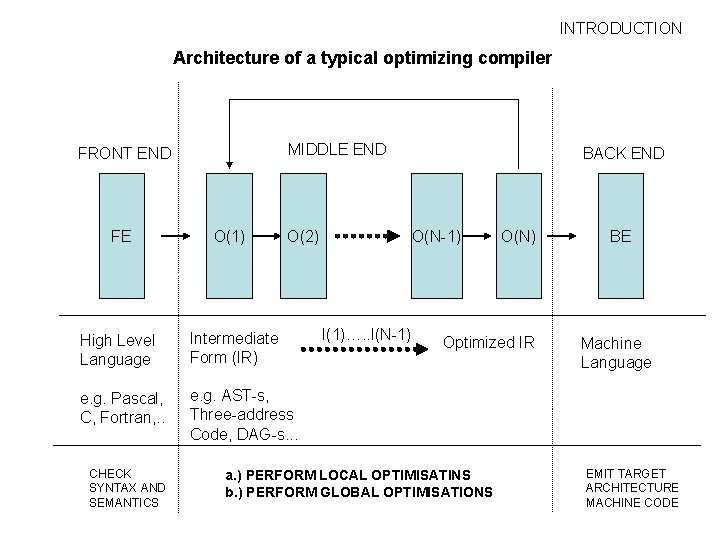
INTRODUCTION Architecture of a typical optimizing compiler MIDDLE END FRONT END FE O(1) High Level Language Intermediate Form (IR) e. g. Pascal, C, Fortran, . . e. g. AST-s, Three-address Code, DAG-s. . . CHECK SYNTAX AND SEMANTICS O(2) BACK END O(N-1) I(1)…. . I(N-1) O(N) Optimized IR a. ) PERFORM LOCAL OPTIMISATINS b. ) PERFORM GLOBAL OPTIMISATIONS BE Machine Language EMIT TARGET ARCHITECTURE MACHINE CODE

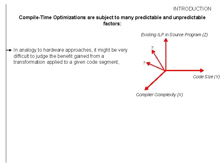
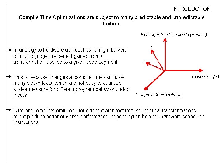
INTRODUCTION Compile-Time Optimizations are subject to many predictable and unpredictable factors: Existing ILP in Source Program (Z) In analogy to hardware approaches, it might be very difficult to judge the benefit gained from a transformation applied to a given code segment, ? ? Code Size (Y) Compiler Complexity (X)

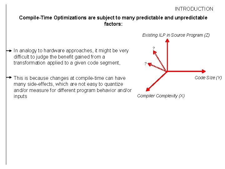
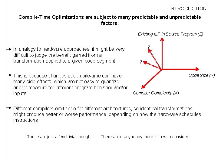
INTRODUCTION Compile-Time Optimizations are subject to many predictable and unpredictable factors: Existing ILP in Source Program (Z) In analogy to hardware approaches, it might be very difficult to judge the benefit gained from a transformation applied to a given code segment, This is because changes at compile-time can have many side-effects, which are not easy to quantize and/or measure for different program behavior and/or inputs ? ? Code Size (Y) Compiler Complexity (X)

INTRODUCTION Compile-Time Optimizations are subject to many predictable and unpredictable factors: Existing ILP in Source Program (Z) In analogy to hardware approaches, it might be very difficult to judge the benefit gained from a transformation applied to a given code segment, This is because changes at compile-time can have many side-effects, which are not easy to quantize and/or measure for different program behavior and/or inputs ? ? Code Size (Y) Compiler Complexity (X) Different compilers emit code for different architectures, so identical transformations might produce better or worse performance, depending on how the hardware schedules instructions

INTRODUCTION Compile-Time Optimizations are subject to many predictable and unpredictable factors: Existing ILP in Source Program (Z) In analogy to hardware approaches, it might be very difficult to judge the benefit gained from a transformation applied to a given code segment, This is because changes at compile-time can have many side-effects, which are not easy to quantize and/or measure for different program behavior and/or inputs ? ? Code Size (Y) Compiler Complexity (X) Different compilers emit code for different architectures, so identical transformations might produce better or worse performance, depending on how the hardware schedules instructions These are just a few trivial thoughts. . There are many more issues to consider!

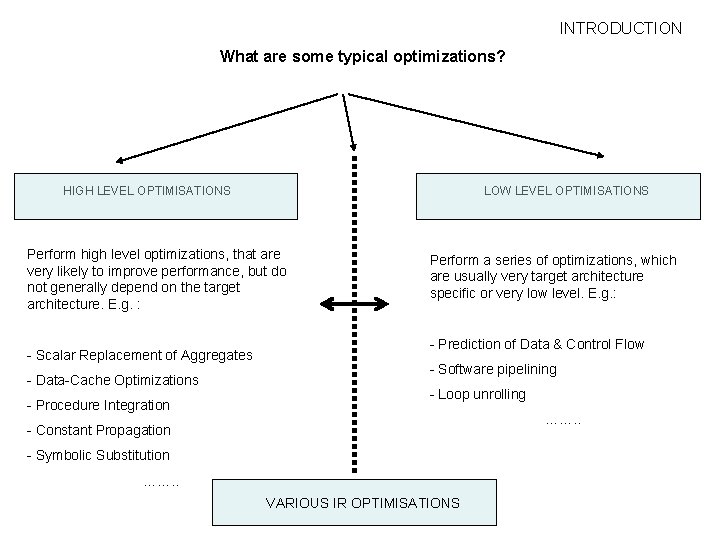
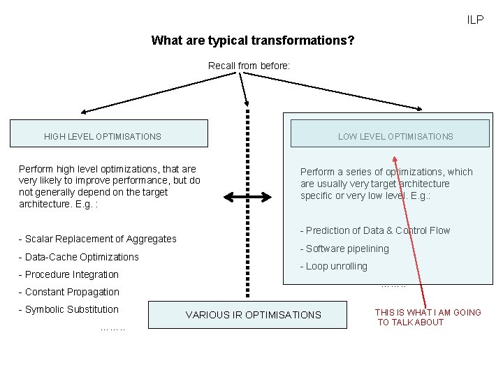
INTRODUCTION What are some typical optimizations? HIGH LEVEL OPTIMISATIONS LOW LEVEL OPTIMISATIONS Perform high level optimizations, that are very likely to improve performance, but do not generally depend on the target architecture. E. g. : - Scalar Replacement of Aggregates - Data-Cache Optimizations - Procedure Integration Perform a series of optimizations, which are usually very target architecture specific or very low level. E. g. : - Prediction of Data & Control Flow - Software pipelining - Loop unrolling ……. . - Constant Propagation - Symbolic Substitution ……. . VARIOUS IR OPTIMISATIONS

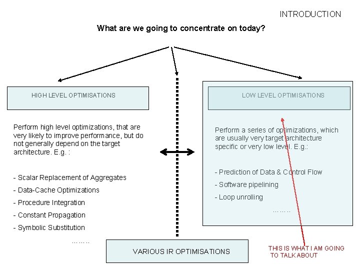
INTRODUCTION What are we going to concentrate on today? HIGH LEVEL OPTIMISATIONS LOW LEVEL OPTIMISATIONS Perform high level optimizations, that are very likely to improve performance, but do not generally depend on the target architecture. E. g. : - Scalar Replacement of Aggregates - Data-Cache Optimizations - Procedure Integration Perform a series of optimizations, which are usually very target architecture specific or very low level. E. g. : - Prediction of Data & Control Flow - Software pipelining - Loop unrolling ……. . - Constant Propagation - Symbolic Substitution ……. . VARIOUS IR OPTIMISATIONS THIS IS WHAT I AM GOING TO TALK ABOUT

Outline 1. Introduction 2. Basic Pipeline Scheduling 3. Instruction Level Parallelism and Dependencies 4. Local Optimizations and Loops 5. Global Scheduling Approaches 6. HW Support for Aggressive Optimization Strategies DONE TALK TALK

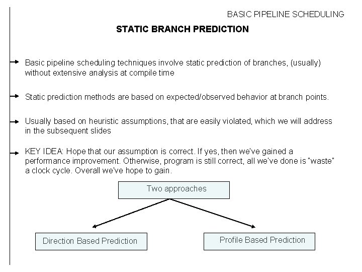
BASIC PIPELINE SCHEDULING STATIC BRANCH PREDICTION Basic pipeline scheduling techniques involve static prediction of branches, (usually) without extensive analysis at compile time

BASIC PIPELINE SCHEDULING STATIC BRANCH PREDICTION Basic pipeline scheduling techniques involve static prediction of branches, (usually) without extensive analysis at compile time Static prediction methods are based on expected/observed behavior at branch points.

BASIC PIPELINE SCHEDULING STATIC BRANCH PREDICTION Basic pipeline scheduling techniques involve static prediction of branches, (usually) without extensive analysis at compile time Static prediction methods are based on expected/observed behavior at branch points. Usually based on heuristic assumptions, that are easily violated, which we will address in the subsequent slides

BASIC PIPELINE SCHEDULING STATIC BRANCH PREDICTION Basic pipeline scheduling techniques involve static prediction of branches, (usually) without extensive analysis at compile time Static prediction methods are based on expected/observed behavior at branch points. Usually based on heuristic assumptions, that are easily violated, which we will address in the subsequent slides KEY IDEA: Hope that our assumption is correct. If yes, then we’ve gained a performance improvement. Otherwise, program is still correct, all we’ve done is “waste” a clock cycle. Overall we’ve hope to gain.

BASIC PIPELINE SCHEDULING STATIC BRANCH PREDICTION Basic pipeline scheduling techniques involve static prediction of branches, (usually) without extensive analysis at compile time Static prediction methods are based on expected/observed behavior at branch points. Usually based on heuristic assumptions, that are easily violated, which we will address in the subsequent slides KEY IDEA: Hope that our assumption is correct. If yes, then we’ve gained a performance improvement. Otherwise, program is still correct, all we’ve done is “waste” a clock cycle. Overall we’ve hope to gain. Two approaches Direction Based Prediction Profile Based Prediction

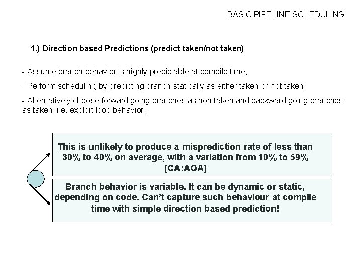
BASIC PIPELINE SCHEDULING 1. ) Direction based Predictions (predict taken/not taken) - Assume branch behavior is highly predictable at compile time, - Perform scheduling by predicting branch statically as either taken or not taken, - Alternatively choose forward going branches as non taken and backward going branches as taken, i. e. exploit loop behavior, This is unlikely to produce a misprediction rate of less than 30% to 40% on average, with a variation from 10% to 59% (CA: AQA) Branch behavior is variable. It can be dynamic or static, depending on code. Can’t capture such behaviour at compile time with simple direction based prediction!

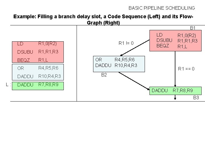
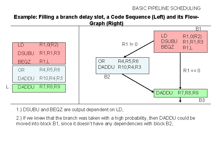
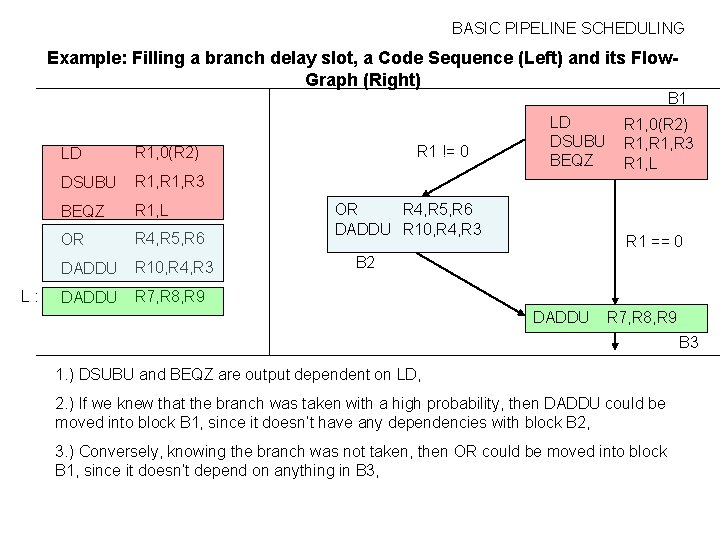
BASIC PIPELINE SCHEDULING Example: Filling a branch delay slot, a Code Sequence (Left) and its Flow. Graph (Right) B 1 L: LD R 1, 0(R 2) DSUBU R 1, R 3 BEQZ R 1, L OR R 4, R 5, R 6 DADDU R 10, R 4, R 3 DADDU R 7, R 8, R 9 R 1 != 0 LD DSUBU BEQZ OR R 4, R 5, R 6 DADDU R 10, R 4, R 3 R 1, 0(R 2) R 1, R 3 R 1, L R 1 == 0 B 2 DADDU R 7, R 8, R 9 B 3

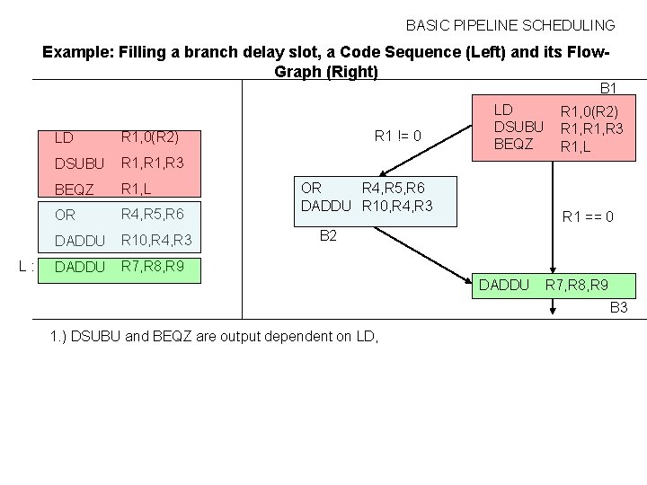
BASIC PIPELINE SCHEDULING Example: Filling a branch delay slot, a Code Sequence (Left) and its Flow. Graph (Right) B 1 L: LD R 1, 0(R 2) DSUBU R 1, R 3 BEQZ R 1, L OR R 4, R 5, R 6 DADDU R 10, R 4, R 3 DADDU R 7, R 8, R 9 R 1 != 0 LD DSUBU BEQZ OR R 4, R 5, R 6 DADDU R 10, R 4, R 3 R 1, 0(R 2) R 1, R 3 R 1, L R 1 == 0 B 2 DADDU R 7, R 8, R 9 B 3 1. ) DSUBU and BEQZ are output dependent on LD,

BASIC PIPELINE SCHEDULING Example: Filling a branch delay slot, a Code Sequence (Left) and its Flow. Graph (Right) B 1 L: LD R 1, 0(R 2) DSUBU R 1, R 3 BEQZ R 1, L OR R 4, R 5, R 6 DADDU R 10, R 4, R 3 DADDU R 7, R 8, R 9 R 1 != 0 LD DSUBU BEQZ OR R 4, R 5, R 6 DADDU R 10, R 4, R 3 R 1, 0(R 2) R 1, R 3 R 1, L R 1 == 0 B 2 DADDU R 7, R 8, R 9 B 3 1. ) DSUBU and BEQZ are output dependent on LD, 2. ) If we knew that the branch was taken with a high probability, then DADDU could be moved into block B 1, since it doesn’t have any dependencies with block B 2,

BASIC PIPELINE SCHEDULING Example: Filling a branch delay slot, a Code Sequence (Left) and its Flow. Graph (Right) B 1 L: LD R 1, 0(R 2) DSUBU R 1, R 3 BEQZ R 1, L OR R 4, R 5, R 6 DADDU R 10, R 4, R 3 DADDU R 7, R 8, R 9 R 1 != 0 LD DSUBU BEQZ OR R 4, R 5, R 6 DADDU R 10, R 4, R 3 R 1, 0(R 2) R 1, R 3 R 1, L R 1 == 0 B 2 DADDU R 7, R 8, R 9 B 3 1. ) DSUBU and BEQZ are output dependent on LD, 2. ) If we knew that the branch was taken with a high probability, then DADDU could be moved into block B 1, since it doesn’t have any dependencies with block B 2, 3. ) Conversely, knowing the branch was not taken, then OR could be moved into block B 1, since it doesn’t depend on anything in B 3,

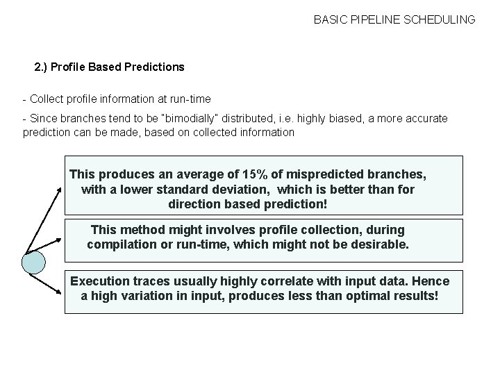
BASIC PIPELINE SCHEDULING 2. ) Profile Based Predictions - Collect profile information at run-time - Since branches tend to be “bimodially” distributed, i. e. highly biased, a more accurate prediction can be made, based on collected information This produces an average of 15% of mispredicted branches, with a lower standard deviation, which is better than for direction based prediction! This method might involves profile collection, during compilation or run-time, which might not be desirable. Execution traces usually highly correlate with input data. Hence a high variation in input, produces less than optimal results!

Outline 1. Introduction 2. Basic Pipeline Scheduling 3. Instruction Level Parallelism and Dependencies 4. Local Optimizations and Loops 5. Global Scheduling Approaches 6. HW Support for Aggressive Optimization Strategies DONE TALK

ILP What is instruction Level Parallelism (ILP)? Inherent property of a sequence of instructions, as a result of which some instructions can be allowed to execute in parallel. (This shall be our definition)

ILP What is instruction Level Parallelism (ILP)? Inherent property of a sequence of instructions, as a result of which some instructions can be allowed to execute in parallel. (This shall be our definition) Note that this definition implies parallelism across a sequence of instruction (block). This could be a loop, a conditional, or some other valid sequence statements.

ILP What is instruction Level Parallelism (ILP)? Inherent property of a sequence of instructions, as a result of which some instructions can be allowed to execute in parallel. (This shall be our definition) Note that this definition implies parallelism across a sequence of instruction (block). This could be a loop, a conditional, or some other valid sequence statements. There is an upper bound, as too how much parallelism can be achieved, since by definition parallelism is an inherent property of a sequence of instructions,

ILP What is instruction Level Parallelism (ILP)? Inherent property of a sequence of instructions, as a result of which some instructions can be allowed to execute in parallel. (This shall be our definition) Note that this definition implies parallelism across a sequence of instruction (block). This could be a loop, a conditional, or some other valid sequence statements. There is an upper bound, as too how much parallelism can be achieved, since by definition parallelism is an inherent property of a sequence of instructions, We can approach this upper bound via a series of transformations, that either expose or allow more ILP to be exposed later transformations

ILP What is instruction Level Parallelism (ILP)? Instruction dependencies within a sequence of instructions determine, how much ILP is present. Think of this as: By what degree can we rearrange the instructions, without compromising correctness?

ILP What is instruction Level Parallelism (ILP)? Instruction dependencies within a sequence of instructions determine, how much ILP is present. Think of this as: By what degree can we rearrange the instructions, without compromising correctness? Hence OUR AIM: Improve performance by exploiting ILP !

ILP How do we exploit ILP? Have a collection of transformations, that operate on or across program blocks, either producing “faster code” or exposing more ILP. Recall from before : An optimizing compiler does this by iteratively applying a series of transformations!

ILP How do we exploit ILP? Have a collection of transformations, that operate on or across program blocks, either producing “faster code” or exposing more ILP. Recall from before : An optimizing compiler does this by iteratively applying a series of transformations! Our transformations should rearrange code, from data available statically at compile time and from the knowledge of the underlying hardware.

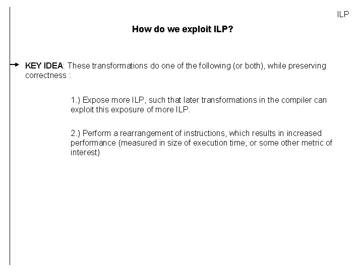
ILP How do we exploit ILP? KEY IDEA: These transformations do one of the following (or both), while preserving correctness : 1. ) Expose more ILP, such that later transformations in the compiler can exploit this exposure of more ILP. 2. ) Perform a rearrangement of instructions, which results in increased performance (measured in size of execution time, or some other metric of interest)

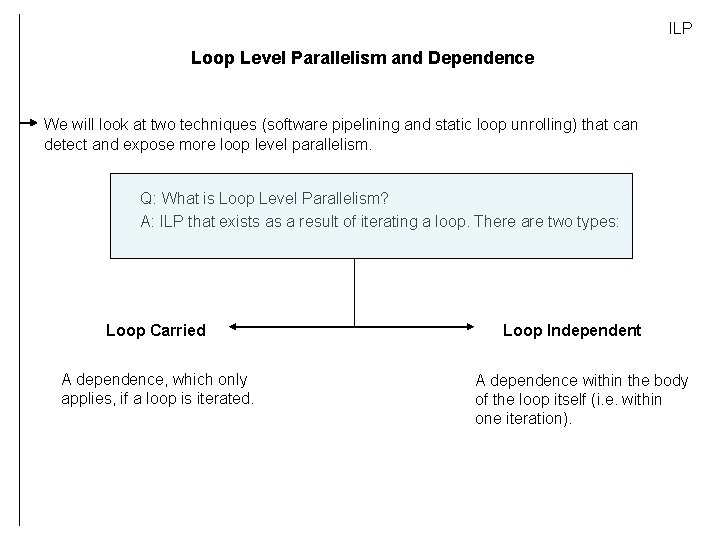
ILP Loop Level Parallelism and Dependence We will look at two techniques (software pipelining and static loop unrolling) that can detect and expose more loop level parallelism. Q: What is Loop Level Parallelism? A: ILP that exists as a result of iterating a loop. There are two types: Loop Carried A dependence, which only applies, if a loop is iterated. Loop Independent A dependence within the body of the loop itself (i. e. within one iteration).

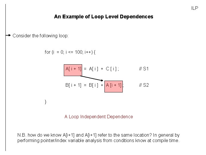
ILP An Example of Loop Level Dependences Consider the following loop: for (i = 0; i <= 100; i++) { A[ i + 1] = A[ i ] + C [ i ] ; // S 1 B[ i + 1] = B[ i ] + A [i + 1] ; // S 2 } A Loop Independent Dependence N. B. how do we know A[i+1] and A[i+1] refer to the same location? In general by performing pointer/index variable analysis from conditions know at compile time.

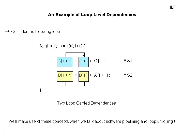
ILP An Example of Loop Level Dependences Consider the following loop: for (i = 0; i <= 100; i++) { A[ i + 1] = A[ i ] + C [ i ] ; // S 1 B[ i + 1] = B[ i ] + A [i + 1] ; // S 2 } Two Loop Carried Dependences We’ll make use of these concepts when we talk about software pipelining and loop unrolling !

ILP What are typical transformations? Recall from before: HIGH LEVEL OPTIMISATIONS LOW LEVEL OPTIMISATIONS Perform high level optimizations, that are very likely to improve performance, but do not generally depend on the target architecture. E. g. : - Scalar Replacement of Aggregates - Data-Cache Optimizations - Procedure Integration Perform a series of optimizations, which are usually very target architecture specific or very low level. E. g. : - Prediction of Data & Control Flow - Software pipelining - Loop unrolling ……. . - Constant Propagation - Symbolic Substitution ……. . VARIOUS IR OPTIMISATIONS THIS IS WHAT I AM GOING TO TALK ABOUT

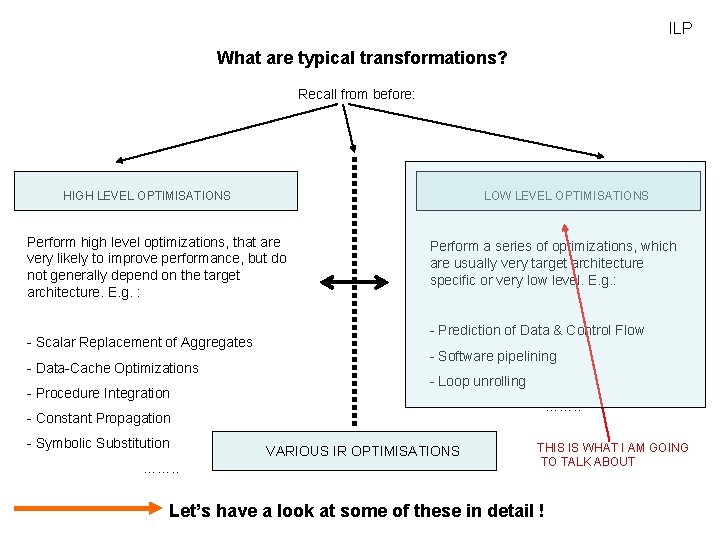
ILP What are typical transformations? Recall from before: HIGH LEVEL OPTIMISATIONS LOW LEVEL OPTIMISATIONS Perform high level optimizations, that are very likely to improve performance, but do not generally depend on the target architecture. E. g. : - Scalar Replacement of Aggregates - Data-Cache Optimizations - Procedure Integration Perform a series of optimizations, which are usually very target architecture specific or very low level. E. g. : - Prediction of Data & Control Flow - Software pipelining - Loop unrolling ……. . - Constant Propagation - Symbolic Substitution ……. . VARIOUS IR OPTIMISATIONS THIS IS WHAT I AM GOING TO TALK ABOUT Let’s have a look at some of these in detail !

Outline 1. Introduction 2. Basic Pipeline Scheduling 3. Instruction Level Parallelism and Dependencies 4. Local Optimizations and Loops 5. Global Scheduling Approaches 6. HW Support for Aggressive Optimization Strategies DONE TALK

LOCAL What is are local transformations? Transformations which operate on basic blocks or extended basic blocks.

LOCAL What is are local transformations? Transformations which operate on basic blocks or extended basic blocks. Our transformations should rearrange code, from data available statically at compile time and from the knowledge of the underlying hardware.

LOCAL What is are local transformations? Transformations which operate on basic blocks or extended basic blocks. Our transformations should rearrange code, from data available statically at compile time and from the knowledge of the underlying hardware. KEY IDEA: These transformations do one of the following (or both), while preserving correctness : 1. ) Expose more ILP, such that later transformations in the compiler can exploit this exposure. 2. ) Perform a rearrangement of instructions, which results in increased performance (measured in size of execution time, or some other metric of interest)

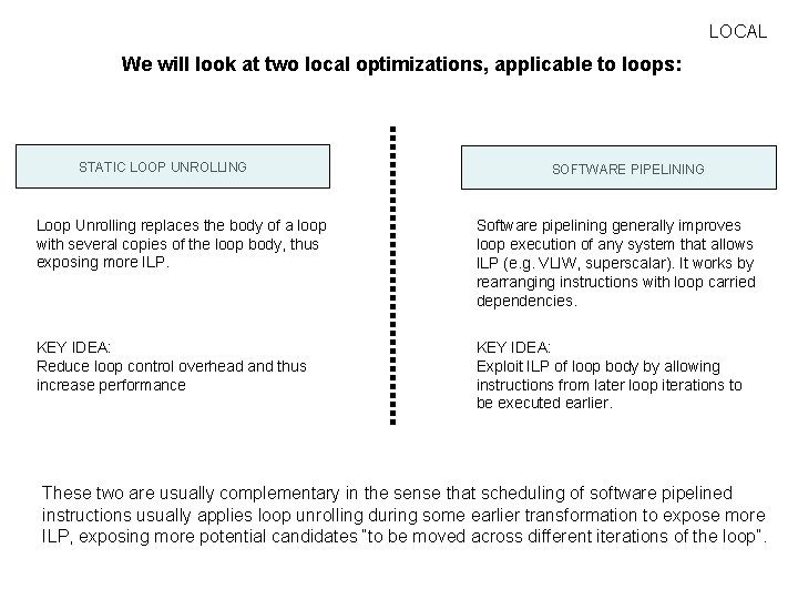
LOCAL We will look at two local optimizations, applicable to loops: STATIC LOOP UNROLLING SOFTWARE PIPELINING Loop Unrolling replaces the body of a loop with several copies of the loop body, thus exposing more ILP. Software pipelining generally improves loop execution of any system that allows ILP (e. g. VLIW, superscalar). It works by rearranging instructions with loop carried dependencies. KEY IDEA: Reduce loop control overhead and thus increase performance KEY IDEA: Exploit ILP of loop body by allowing instructions from later loop iterations to be executed earlier. These two are usually complementary in the sense that scheduling of software pipelined instructions usually applies loop unrolling during some earlier transformation to expose more ILP, exposing more potential candidates “to be moved across different iterations of the loop”.

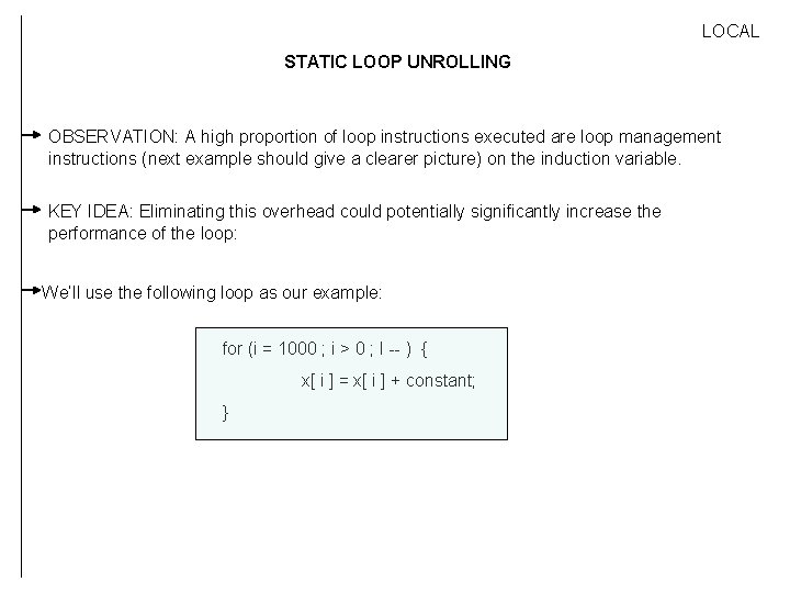
LOCAL STATIC LOOP UNROLLING OBSERVATION: A high proportion of loop instructions executed are loop management instructions (next example should give a clearer picture) on the induction variable.

LOCAL STATIC LOOP UNROLLING OBSERVATION: A high proportion of loop instructions executed are loop management instructions (next example should give a clearer picture) on the induction variable. KEY IDEA: Eliminating this overhead could potentially significantly increase the performance of the loop:

LOCAL STATIC LOOP UNROLLING OBSERVATION: A high proportion of loop instructions executed are loop management instructions (next example should give a clearer picture) on the induction variable. KEY IDEA: Eliminating this overhead could potentially significantly increase the performance of the loop: We’ll use the following loop as our example: for (i = 1000 ; i > 0 ; I -- ) { x[ i ] = x[ i ] + constant; }

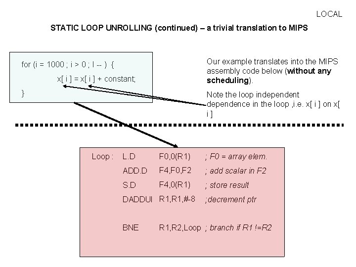
LOCAL STATIC LOOP UNROLLING (continued) – a trivial translation to MIPS Our example translates into the MIPS assembly code below (without any scheduling). for (i = 1000 ; i > 0 ; I -- ) { x[ i ] = x[ i ] + constant; } Note the loop independent dependence in the loop , i. e. x[ i ] on x[ i] Loop : L. D F 0, 0(R 1) ; F 0 = array elem. ADD. D F 4, F 0, F 2 ; add scalar in F 2 S. D F 4, 0(R 1) ; store result DADDUI R 1, #-8 BNE ; decrement ptr R 1, R 2, Loop ; branch if R 1 !=R 2

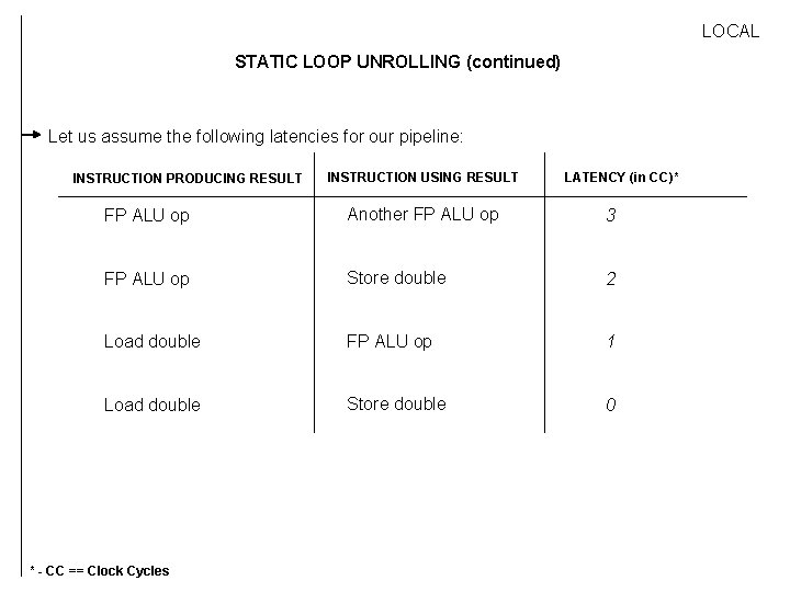
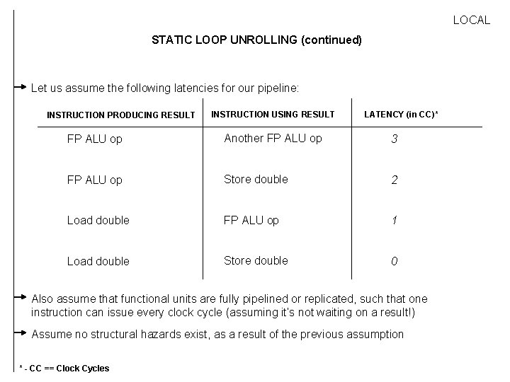
LOCAL STATIC LOOP UNROLLING (continued) Let us assume the following latencies for our pipeline: INSTRUCTION PRODUCING RESULT INSTRUCTION USING RESULT LATENCY (in CC)* FP ALU op Another FP ALU op 3 FP ALU op Store double 2 Load double FP ALU op 1 Load double Store double 0 * - CC == Clock Cycles

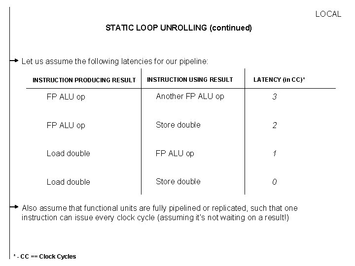
LOCAL STATIC LOOP UNROLLING (continued) Let us assume the following latencies for our pipeline: INSTRUCTION PRODUCING RESULT INSTRUCTION USING RESULT LATENCY (in CC)* FP ALU op Another FP ALU op 3 FP ALU op Store double 2 Load double FP ALU op 1 Load double Store double 0 Also assume that functional units are fully pipelined or replicated, such that one instruction can issue every clock cycle (assuming it’s not waiting on a result!) * - CC == Clock Cycles

LOCAL STATIC LOOP UNROLLING (continued) Let us assume the following latencies for our pipeline: INSTRUCTION PRODUCING RESULT INSTRUCTION USING RESULT LATENCY (in CC)* FP ALU op Another FP ALU op 3 FP ALU op Store double 2 Load double FP ALU op 1 Load double Store double 0 Also assume that functional units are fully pipelined or replicated, such that one instruction can issue every clock cycle (assuming it’s not waiting on a result!) Assume no structural hazards exist, as a result of the previous assumption * - CC == Clock Cycles

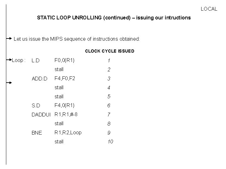
LOCAL STATIC LOOP UNROLLING (continued) – issuing our intructions Let us issue the MIPS sequence of instructions obtained: CLOCK CYCLE ISSUED Loop : L. D ADD. D S. D F 0, 0(R 1) 1 stall 2 F 4, F 0, F 2 3 stall 4 stall 5 F 4, 0(R 1) 6 DADDUI R 1, #-8 BNE 7 stall 8 R 1, R 2, Loop 9 stall 10

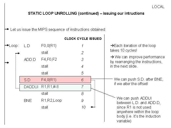
LOCAL STATIC LOOP UNROLLING (continued) – issuing our intructions Let us issue the MIPS sequence of instructions obtained: CLOCK CYCLE ISSUED Loop : L. D ADD. D S. D F 0, 0(R 1) 1 stall 2 F 4, F 0, F 2 3 stall 4 stall 5 F 4, 0(R 1) 6 DADDUI R 1, #-8 BNE 7 stall 8 R 1, R 2, Loop 9 stall 10 Each iteration of the loop takes 10 cycles! We can improve performance by rearranging the instructions, in the next slide. We can push S. D. after BNE, if we alter the offset! We can push ADDUI between L. D. and ADD. D, since R 1 is not used anywhere within the loop body (i. e. it’s the induction variable)

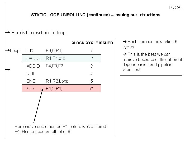
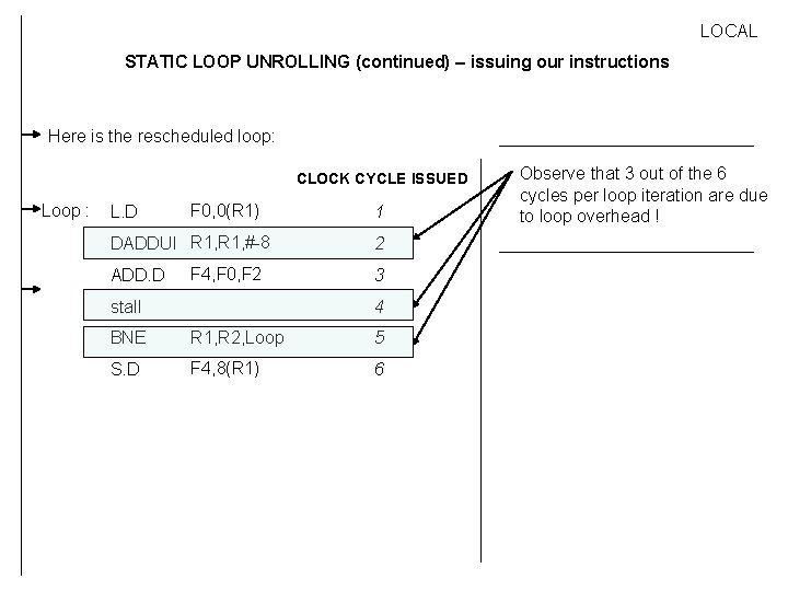
LOCAL STATIC LOOP UNROLLING (continued) – issuing our intructions Here is the rescheduled loop: CLOCK CYCLE ISSUED Loop : L. D F 0, 0(R 1) DADDUI R 1, #-8 ADD. D F 4, F 0, F 2 stall 1 2 3 4 BNE R 1, R 2, Loop 5 S. D F 4, 8(R 1) 6 Here we’ve decremented R 1 before we’ve stored F 4. Hence need an offset of 8! Each iteration now takes 6 cycles This is the best we can achieve because of the inherent dependencies and pipeline latencies!

LOCAL STATIC LOOP UNROLLING (continued) – issuing our instructions Here is the rescheduled loop: CLOCK CYCLE ISSUED Loop : L. D F 0, 0(R 1) DADDUI R 1, #-8 ADD. D F 4, F 0, F 2 stall 1 2 3 4 BNE R 1, R 2, Loop 5 S. D F 4, 8(R 1) 6 Observe that 3 out of the 6 cycles per loop iteration are due to loop overhead !

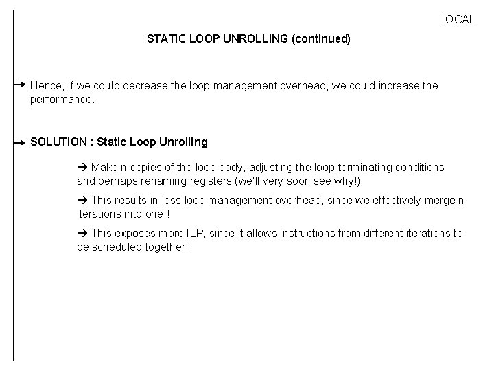
LOCAL STATIC LOOP UNROLLING (continued) Hence, if we could decrease the loop management overhead, we could increase the performance. SOLUTION : Static Loop Unrolling

LOCAL STATIC LOOP UNROLLING (continued) Hence, if we could decrease the loop management overhead, we could increase the performance. SOLUTION : Static Loop Unrolling Make n copies of the loop body, adjusting the loop terminating conditions and perhaps renaming registers (we’ll very soon see why!),

LOCAL STATIC LOOP UNROLLING (continued) Hence, if we could decrease the loop management overhead, we could increase the performance. SOLUTION : Static Loop Unrolling Make n copies of the loop body, adjusting the loop terminating conditions and perhaps renaming registers (we’ll very soon see why!), This results in less loop management overhead, since we effectively merge n iterations into one !

LOCAL STATIC LOOP UNROLLING (continued) Hence, if we could decrease the loop management overhead, we could increase the performance. SOLUTION : Static Loop Unrolling Make n copies of the loop body, adjusting the loop terminating conditions and perhaps renaming registers (we’ll very soon see why!), This results in less loop management overhead, since we effectively merge n iterations into one ! This exposes more ILP, since it allows instructions from different iterations to be scheduled together!

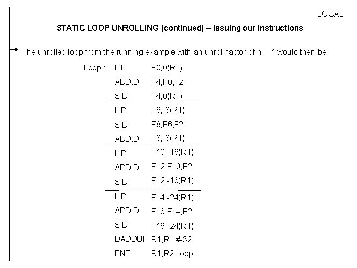
LOCAL STATIC LOOP UNROLLING (continued) – issuing our instructions The unrolled loop from the running example with an unroll factor of n = 4 would then be: Loop : L. D F 0, 0(R 1) ADD. D F 4, F 0, F 2 S. D F 4, 0(R 1) L. D F 6, -8(R 1) S. D F 8, F 6, F 2 ADD. D F 8, -8(R 1) L. D F 10, -16(R 1) ADD. D F 12, F 10, F 2 S. D F 12, -16(R 1) L. D F 14, -24(R 1) ADD. D F 16, F 14, F 2 S. D F 16, -24(R 1) DADDUI R 1, #-32 BNE R 1, R 2, Loop

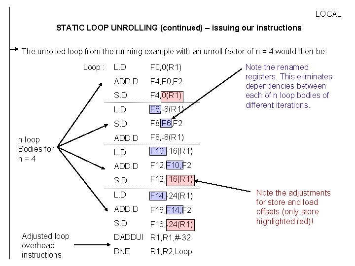
LOCAL STATIC LOOP UNROLLING (continued) – issuing our instructions The unrolled loop from the running example with an unroll factor of n = 4 would then be: Loop : n loop Bodies for n=4 Adjusted loop overhead instructions L. D F 0, 0(R 1) ADD. D F 4, F 0, F 2 S. D F 4, 0(R 1) L. D F 6, -8(R 1) S. D F 8, F 6, F 2 ADD. D F 8, -8(R 1) L. D F 10, -16(R 1) ADD. D F 12, F 10, F 2 S. D F 12, -16(R 1) L. D F 14, -24(R 1) ADD. D F 16, F 14, F 2 S. D F 16, -24(R 1) DADDUI R 1, #-32 BNE R 1, R 2, Loop Note the renamed registers. This eliminates dependencies between each of n loop bodies of different iterations. Note the adjustments for store and load offsets (only store highlighted red)!

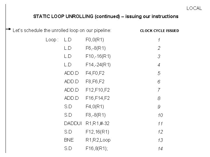
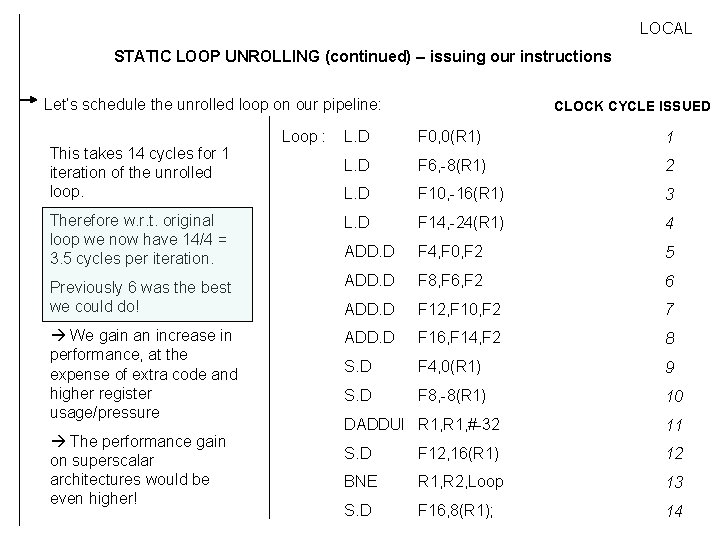
LOCAL STATIC LOOP UNROLLING (continued) – issuing our instructions Let’s schedule the unrolled loop on our pipeline: Loop : CLOCK CYCLE ISSUED L. D F 0, 0(R 1) 1 L. D F 6, -8(R 1) 2 L. D F 10, -16(R 1) 3 L. D F 14, -24(R 1) 4 ADD. D F 4, F 0, F 2 5 ADD. D F 8, F 6, F 2 6 ADD. D F 12, F 10, F 2 7 ADD. D F 16, F 14, F 2 8 S. D F 4, 0(R 1) 9 S. D F 8, -8(R 1) 10 DADDUI R 1, #-32 11 S. D F 12, 16(R 1) 12 BNE R 1, R 2, Loop 13 S. D F 16, 8(R 1); 14

LOCAL STATIC LOOP UNROLLING (continued) – issuing our instructions Let’s schedule the unrolled loop on our pipeline: Loop : CLOCK CYCLE ISSUED L. D F 0, 0(R 1) 1 L. D F 6, -8(R 1) 2 L. D F 10, -16(R 1) 3 Therefore w. r. t. original loop we now have 14/4 = 3. 5 cycles per iteration. L. D F 14, -24(R 1) 4 ADD. D F 4, F 0, F 2 5 Previously 6 was the best we could do! ADD. D F 8, F 6, F 2 6 ADD. D F 12, F 10, F 2 7 We gain an increase in performance, at the expense of extra code and higher register usage/pressure ADD. D F 16, F 14, F 2 8 S. D F 4, 0(R 1) 9 S. D F 8, -8(R 1) 10 This takes 14 cycles for 1 iteration of the unrolled loop. The performance gain on superscalar architectures would be even higher! DADDUI R 1, #-32 11 S. D F 12, 16(R 1) 12 BNE R 1, R 2, Loop 13 S. D F 16, 8(R 1); 14

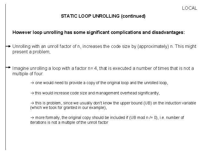
LOCAL STATIC LOOP UNROLLING (continued) However loop unrolling has some significant complications and disadvantages: Unrolling with an unroll factor of n, increases the code size by (approximately) n. This might present a problem,

LOCAL STATIC LOOP UNROLLING (continued) However loop unrolling has some significant complications and disadvantages: Unrolling with an unroll factor of n, increases the code size by (approximately) n. This might present a problem, Imagine unrolling a loop with a factor n= 4, that is executed a number of times that is not a multiple of four: one would need to provide a copy of the original loop and the unrolled loop, this would increase code size and management overhead significantly, this is problem, since we usually don’t know the upper bound (UB) on the induction variable (which we took for granted in our example), more formally, the original copy should be included if (UB mod n /= 0), i. e. number of iterations is not a multiple of the unroll factor

LOCAL STATIC LOOP UNROLLING (continued) However loop unrolling has some significant complications and disadvantages: We usually need to perform register renaming, such that we decrease dependencies within the unrolled loop. This increases the register pressure!

LOCAL STATIC LOOP UNROLLING (continued) However loop unrolling has some significant complications and disadvantages: We usually need to perform register renaming, such that we decrease dependencies within the unrolled loop. This increases the register pressure! The criteria for performing loop unrolling are usually very restrictive!

LOCAL SOFTWARE PIPELINING Software Pipelining is an optimization that can improve the loop-execution-performance of any system that allows ILP, including VLIW and superscalar architectures,

LOCAL SOFTWARE PIPELINING Software Pipelining is an optimization that can improve the loop-execution-performance of any system that allows ILP, including VLIW and superscalar architectures, It derives its performance gain by filling delays within each iteration of a loop body with instructions from different iterations of that same loop,

LOCAL SOFTWARE PIPELINING Software Pipelining is an optimization that can improve the loop-execution-performance of any system that allows ILP, including VLIW and superscalar architectures, It derives its performance gain by filling delays within each iteration of a loop body with instructions from different iterations of that same loop, This method requires fewer registers per loop iteration than loop unrolling,

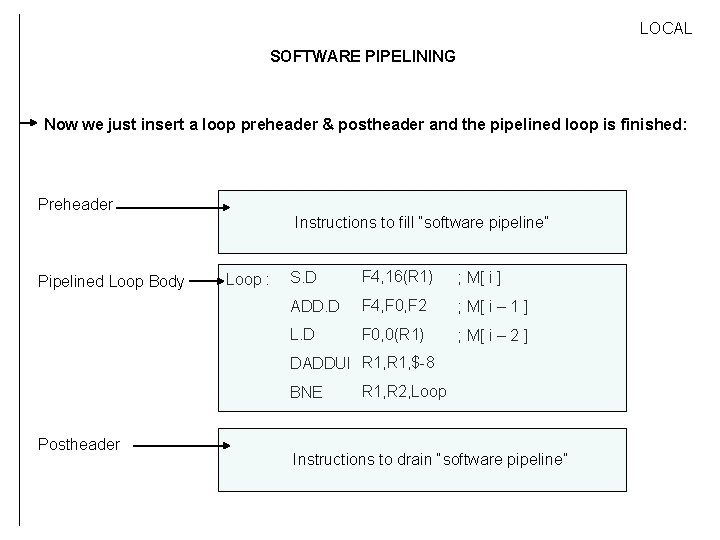
LOCAL SOFTWARE PIPELINING Software Pipelining is an optimization that can improve the loop-execution-performance of any system that allows ILP, including VLIW and superscalar architectures, It derives its performance gain by filling delays within each iteration of a loop body with instructions from different iterations of that same loop, This method requires fewer registers per loop iteration than loop unrolling, This method requires some extra code to fill (preheader) and drain (postheader) the software pipelined loop, as we’ll see in the next example.

LOCAL SOFTWARE PIPELINING Software Pipelining is an optimization that can improve the loop-execution-performance of any system that allows ILP, including VLIW and superscalar architectures, It derives its performance gain by filling delays within each iteration of a loop body with instructions from different iterations of that same loop, This method requires fewer registers per loop iteration than loop unrolling, This method requires some extra code to fill (preheader) and drain (postheader) the software pipelined loop, as we’ll see in the next example. KEY IDEA: Increase performance by scheduling instructions from different iterations within inside the same loop body.

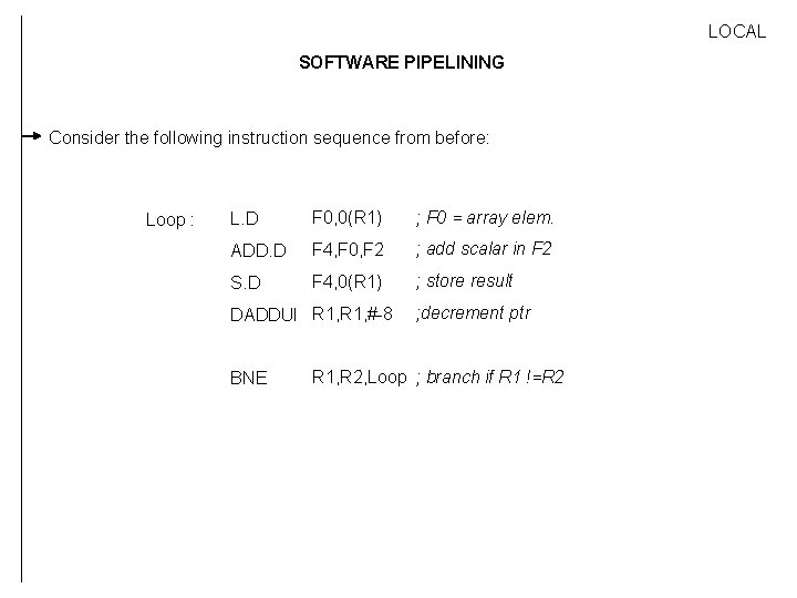
LOCAL SOFTWARE PIPELINING Consider the following instruction sequence from before: Loop : L. D F 0, 0(R 1) ; F 0 = array elem. ADD. D F 4, F 0, F 2 ; add scalar in F 2 S. D F 4, 0(R 1) ; store result DADDUI R 1, #-8 BNE ; decrement ptr R 1, R 2, Loop ; branch if R 1 !=R 2

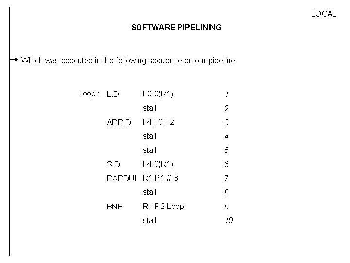
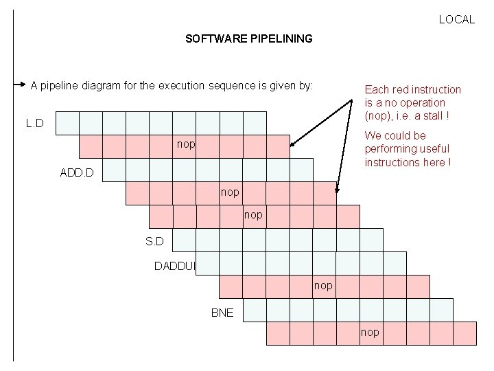
LOCAL SOFTWARE PIPELINING Which was executed in the following sequence on our pipeline: Loop : L. D ADD. D S. D F 0, 0(R 1) 1 stall 2 F 4, F 0, F 2 3 stall 4 stall 5 F 4, 0(R 1) 6 DADDUI R 1, #-8 BNE 7 stall 8 R 1, R 2, Loop 9 stall 10

LOCAL SOFTWARE PIPELINING A pipeline diagram for the execution sequence is given by: Each red instruction is a no operation (nop), i. e. a stall ! L. D We could be performing useful instructions here ! nop ADD. D nop S. D DADDUI nop BNE nop

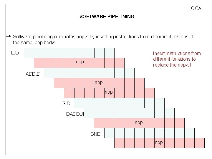
LOCAL SOFTWARE PIPELINING Software pipelining eliminates nop-s by inserting instructions from different iterations of the same loop body: L. D Insert instructions from different iterations to replace the nop-s! nop ADD. D nop S. D DADDUI nop BNE nop

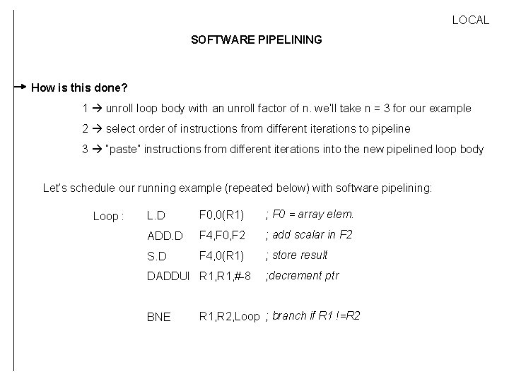
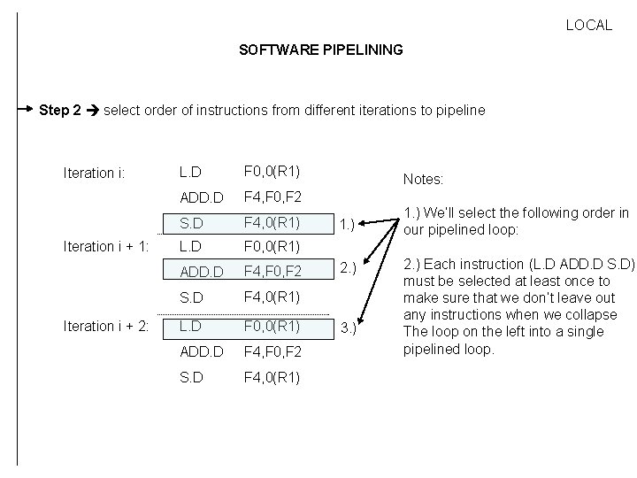
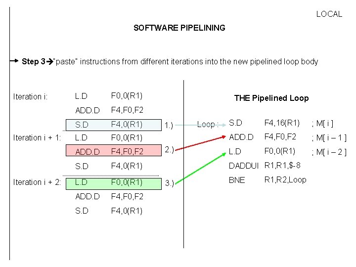
LOCAL SOFTWARE PIPELINING How is this done? 1 unroll loop body with an unroll factor of n. we’ll take n = 3 for our example 2 select order of instructions from different iterations to pipeline 3 “paste” instructions from different iterations into the new pipelined loop body Let’s schedule our running example (repeated below) with software pipelining: Loop : L. D F 0, 0(R 1) ; F 0 = array elem. ADD. D F 4, F 0, F 2 ; add scalar in F 2 S. D F 4, 0(R 1) ; store result DADDUI R 1, #-8 BNE ; decrement ptr R 1, R 2, Loop ; branch if R 1 !=R 2

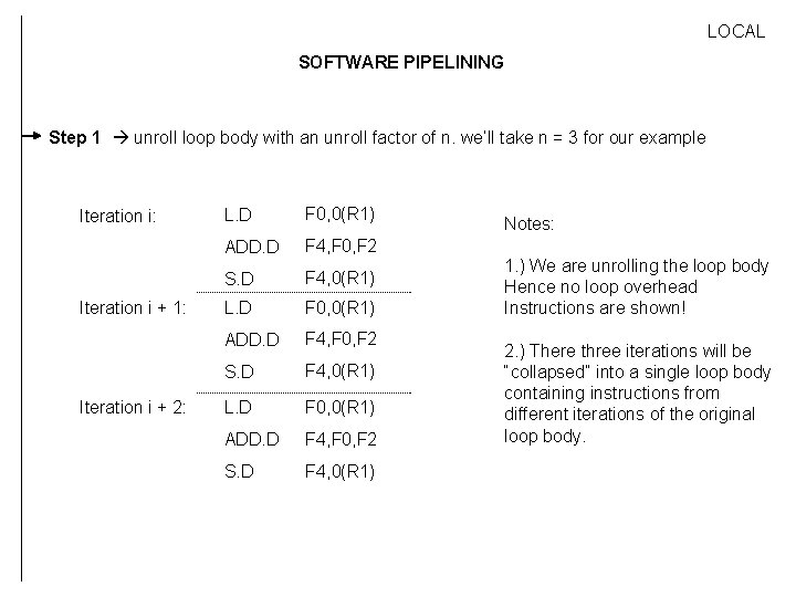
LOCAL SOFTWARE PIPELINING Step 1 unroll loop body with an unroll factor of n. we’ll take n = 3 for our example Iteration i: Iteration i + 1: Iteration i + 2: L. D F 0, 0(R 1) ADD. D F 4, F 0, F 2 S. D F 4, 0(R 1) Notes: 1. ) We are unrolling the loop body Hence no loop overhead Instructions are shown! 2. ) There three iterations will be “collapsed” into a single loop body containing instructions from different iterations of the original loop body.

LOCAL SOFTWARE PIPELINING Step 2 select order of instructions from different iterations to pipeline Iteration i: Iteration i + 1: Iteration i + 2: L. D F 0, 0(R 1) ADD. D F 4, F 0, F 2 S. D F 4, 0(R 1) Notes: 1. ) 2. ) 3. ) 1. ) We’ll select the following order in our pipelined loop: 2. ) Each instruction (L. D ADD. D S. D) must be selected at least once to make sure that we don’t leave out any instructions when we collapse The loop on the left into a single pipelined loop.

LOCAL SOFTWARE PIPELINING Step 3 “paste” instructions from different iterations into the new pipelined loop body Iteration i: Iteration i + 1: Iteration i + 2: L. D F 0, 0(R 1) ADD. D F 4, F 0, F 2 S. D F 4, 0(R 1) THE Pipelined Loop 1. ) 2. ) Loop : S. D F 4, 16(R 1) ; M[ i ] ADD. D F 4, F 0, F 2 ; M[ i – 1 ] L. D F 0, 0(R 1) ; M[ i – 2 ] DADDUI R 1, $-8 3. ) BNE R 1, R 2, Loop

LOCAL SOFTWARE PIPELINING Now we just insert a loop preheader & postheader and the pipelined loop is finished: Preheader Instructions to fill “software pipeline” Pipelined Loop Body Loop : S. D F 4, 16(R 1) ; M[ i ] ADD. D F 4, F 0, F 2 ; M[ i – 1 ] L. D F 0, 0(R 1) ; M[ i – 2 ] DADDUI R 1, $-8 BNE Postheader R 1, R 2, Loop Instructions to drain “software pipeline”

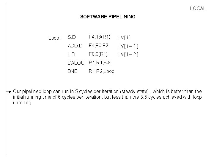
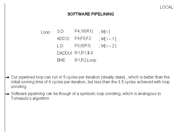
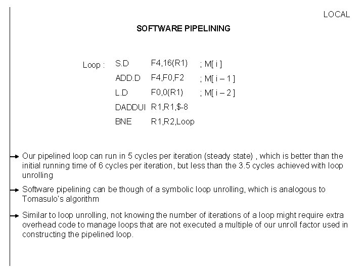
LOCAL SOFTWARE PIPELINING Loop : S. D F 4, 16(R 1) ; M[ i ] ADD. D F 4, F 0, F 2 ; M[ i – 1 ] L. D F 0, 0(R 1) ; M[ i – 2 ] DADDUI R 1, $-8 BNE R 1, R 2, Loop Our pipelined loop can run in 5 cycles per iteration (steady state) , which is better than the initial running time of 6 cycles per iteration, but less than the 3. 5 cycles achieved with loop unrolling

LOCAL SOFTWARE PIPELINING Loop : S. D F 4, 16(R 1) ; M[ i ] ADD. D F 4, F 0, F 2 ; M[ i – 1 ] L. D F 0, 0(R 1) ; M[ i – 2 ] DADDUI R 1, $-8 BNE R 1, R 2, Loop Our pipelined loop can run in 5 cycles per iteration (steady state) , which is better than the initial running time of 6 cycles per iteration, but less than the 3. 5 cycles achieved with loop unrolling Software pipelining can be though of a symbolic loop unrolling, which is analogous to Tomasulo’s algorithm

LOCAL SOFTWARE PIPELINING Loop : S. D F 4, 16(R 1) ; M[ i ] ADD. D F 4, F 0, F 2 ; M[ i – 1 ] L. D F 0, 0(R 1) ; M[ i – 2 ] DADDUI R 1, $-8 BNE R 1, R 2, Loop Our pipelined loop can run in 5 cycles per iteration (steady state) , which is better than the initial running time of 6 cycles per iteration, but less than the 3. 5 cycles achieved with loop unrolling Software pipelining can be though of a symbolic loop unrolling, which is analogous to Tomasulo’s algorithm Similar to loop unrolling, not knowing the number of iterations of a loop might require extra overhead code to manage loops that are not executed a multiple of our unroll factor used in constructing the pipelined loop.

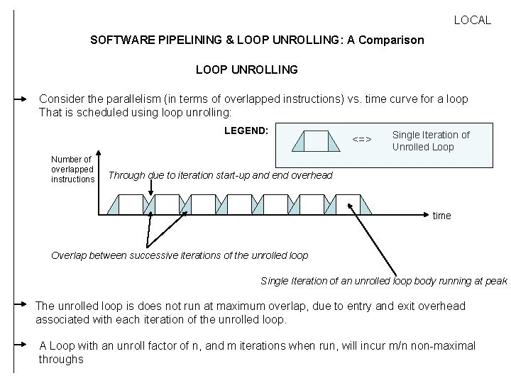
LOCAL SOFTWARE PIPELINING & LOOP UNROLLING: A Comparison LOOP UNROLLING Consider the parallelism (in terms of overlapped instructions) vs. time curve for a loop That is scheduled using loop unrolling: LEGEND: Number of overlapped instructions <=> Single Iteration of Unrolled Loop Through due to iteration start-up and end overhead time Overlap between successive iterations of the unrolled loop Single Iteration of an unrolled loop body running at peak The unrolled loop is does not run at maximum overlap, due to entry and exit overhead associated with each iteration of the unrolled loop. A Loop with an unroll factor of n, and m iterations when run, will incur m/n non-maximal throughs

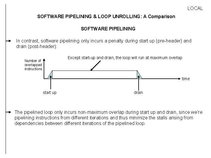
LOCAL SOFTWARE PIPELINING & LOOP UNROLLING: A Comparison SOFTWARE PIPELINING In contrast, software pipelining only incurs a penalty during start up (pre-header) and drain (post-header): Except start-up and drain, the loop will run at maximum overlap Number of overlapped instructions time start up drain The pipelined loop only incurs non-maximum overlap during start up and drain, since we’re pipelining instructions from different iterations and thus minimize the stalls arising from dependencies between different iterations of the pipelined loop.

Outline 1. Introduction 2. Basic Pipeline Scheduling 3. Instruction Level Parallelism and Dependencies 4. Local Optimizations and Loops 5. Global Scheduling Approaches 6. HW Support for Aggressive Optimization Strategies DONE TALK

GLOBAL Global Scheduling Approaches The Approaches seen so far work well with linear code segments,

GLOBAL Global Scheduling Approaches The Approaches seen so far work well with linear code segments, For programs with more complex control flow (i. e. more branching), our approaches so far would not very effective, since we cannot move code across (non-LOOP) branches,

GLOBAL Global Scheduling Approaches The Approaches seen so far work well with linear code segments, For programs with more complex control flow (i. e. more branching), our approaches so far would not very effective, since we cannot move code across (non-LOOP) branches, Hence we would ideally like to be able to move instructions across branches,

GLOBAL Global Scheduling Approaches The Approaches seen so far work well with linear code segments, For programs with more complex control flow (i. e. more branching), our approaches so far would not very effective, since we cannot move code across (non-LOOP) branches, Hence we would ideally like to be able to move instructions across branches, Global scheduling approaches perform code movement across branches, based on the relative frequency of execution across different control flow paths,

GLOBAL Global Scheduling Approaches The Approaches seen so far work well with linear code segments, For programs with more complex control flow (i. e. more branching), our approaches so far would not very effective, since we cannot move code across (non-LOOP) branches, Hence we would ideally like to be able to move instructions across branches, Global scheduling approaches perform code movement across branches, based on the relative frequency of execution across different control flow paths, This approach must deal with both control dependencies (on branches) and data dependencies that exist both within and across basic blocks,

GLOBAL Global Scheduling Approaches The Approaches seen so far work well with linear code segments, For programs with more complex control flow (i. e. more branching), our approaches so far would not very effective, since we cannot move code across (non-LOOP) branches, Hence we would ideally like to be able to move instructions across branches, Global scheduling approaches perform code movement across branches, based on the relative frequency of execution across different control flow paths, This approach must deal with both control dependencies (on branches) and data dependencies that exist both within and across basic blocks, Since static global scheduling is subject to numerous constraints, hardware approaches exist for either eliminating (multiple-issue Tomasulo) or supporting compile time scheduling, as we’ll see in the next section.

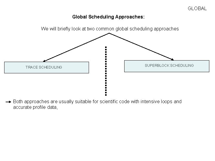
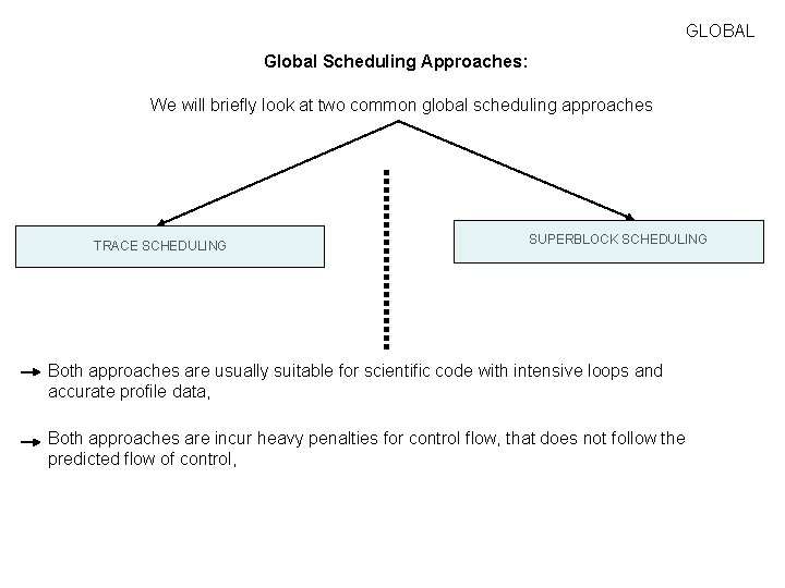
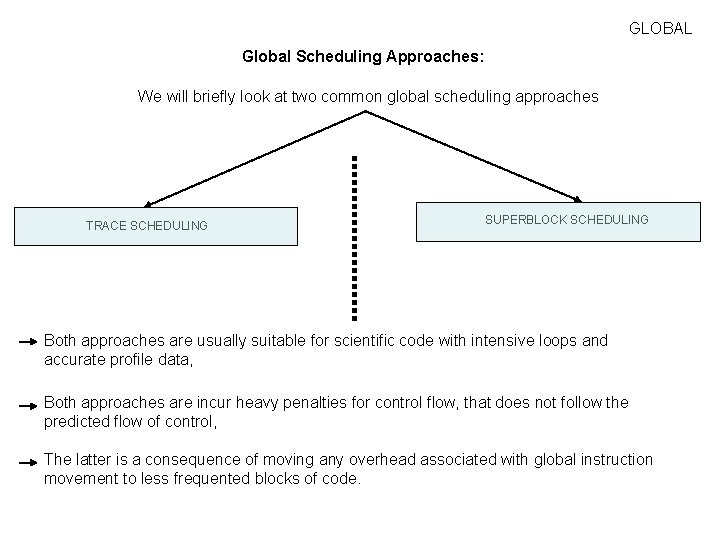
GLOBAL Global Scheduling Approaches: We will briefly look at two common global scheduling approaches TRACE SCHEDULING SUPERBLOCK SCHEDULING

GLOBAL Global Scheduling Approaches: We will briefly look at two common global scheduling approaches TRACE SCHEDULING SUPERBLOCK SCHEDULING Both approaches are usually suitable for scientific code with intensive loops and accurate profile data,

GLOBAL Global Scheduling Approaches: We will briefly look at two common global scheduling approaches TRACE SCHEDULING SUPERBLOCK SCHEDULING Both approaches are usually suitable for scientific code with intensive loops and accurate profile data, Both approaches are incur heavy penalties for control flow, that does not follow the predicted flow of control,

GLOBAL Global Scheduling Approaches: We will briefly look at two common global scheduling approaches TRACE SCHEDULING SUPERBLOCK SCHEDULING Both approaches are usually suitable for scientific code with intensive loops and accurate profile data, Both approaches are incur heavy penalties for control flow, that does not follow the predicted flow of control, The latter is a consequence of moving any overhead associated with global instruction movement to less frequented blocks of code.

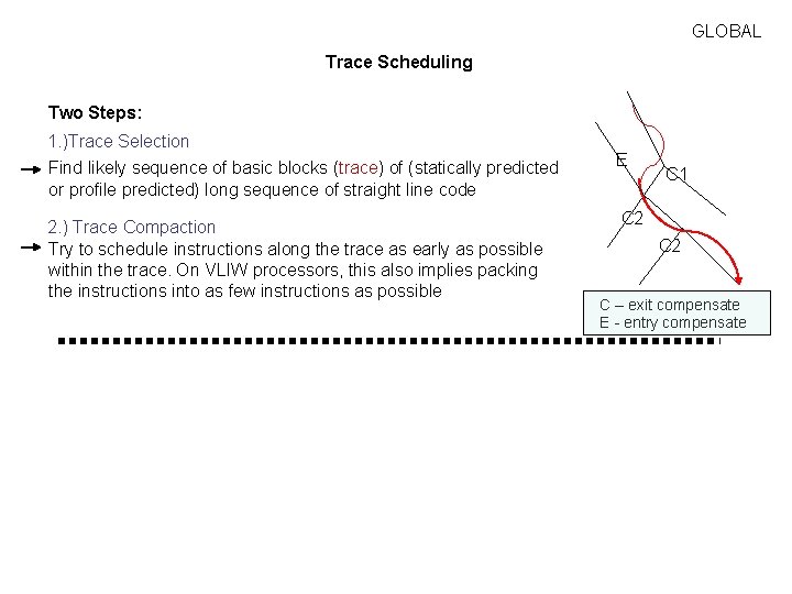
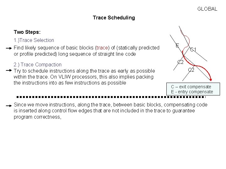
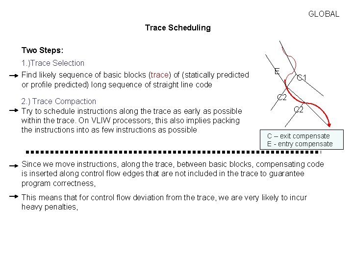
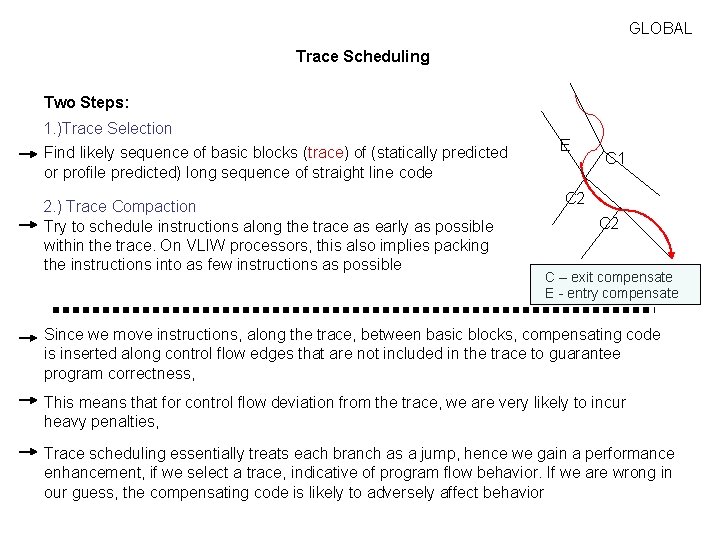
GLOBAL Trace Scheduling Two Steps: 1. )Trace Selection Find likely sequence of basic blocks (trace) of (statically predicted or profile predicted) long sequence of straight line code 2. ) Trace Compaction Try to schedule instructions along the trace as early as possible within the trace. On VLIW processors, this also implies packing the instructions into as few instructions as possible E C 1 C 2 C – exit compensate E - entry compensate

GLOBAL Trace Scheduling Two Steps: 1. )Trace Selection Find likely sequence of basic blocks (trace) of (statically predicted or profile predicted) long sequence of straight line code 2. ) Trace Compaction Try to schedule instructions along the trace as early as possible within the trace. On VLIW processors, this also implies packing the instructions into as few instructions as possible E C 1 C 2 C – exit compensate E - entry compensate Since we move instructions, along the trace, between basic blocks, compensating code is inserted along control flow edges that are not included in the trace to guarantee program correctness,

GLOBAL Trace Scheduling Two Steps: 1. )Trace Selection Find likely sequence of basic blocks (trace) of (statically predicted or profile predicted) long sequence of straight line code 2. ) Trace Compaction Try to schedule instructions along the trace as early as possible within the trace. On VLIW processors, this also implies packing the instructions into as few instructions as possible E C 1 C 2 C – exit compensate E - entry compensate Since we move instructions, along the trace, between basic blocks, compensating code is inserted along control flow edges that are not included in the trace to guarantee program correctness, This means that for control flow deviation from the trace, we are very likely to incur heavy penalties,

GLOBAL Trace Scheduling Two Steps: 1. )Trace Selection Find likely sequence of basic blocks (trace) of (statically predicted or profile predicted) long sequence of straight line code 2. ) Trace Compaction Try to schedule instructions along the trace as early as possible within the trace. On VLIW processors, this also implies packing the instructions into as few instructions as possible E C 1 C 2 C – exit compensate E - entry compensate Since we move instructions, along the trace, between basic blocks, compensating code is inserted along control flow edges that are not included in the trace to guarantee program correctness, This means that for control flow deviation from the trace, we are very likely to incur heavy penalties, Trace scheduling essentially treats each branch as a jump, hence we gain a performance enhancement, if we select a trace, indicative of program flow behavior. If we are wrong in our guess, the compensating code is likely to adversely affect behavior

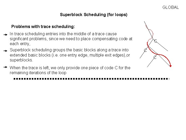
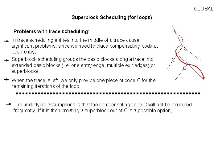
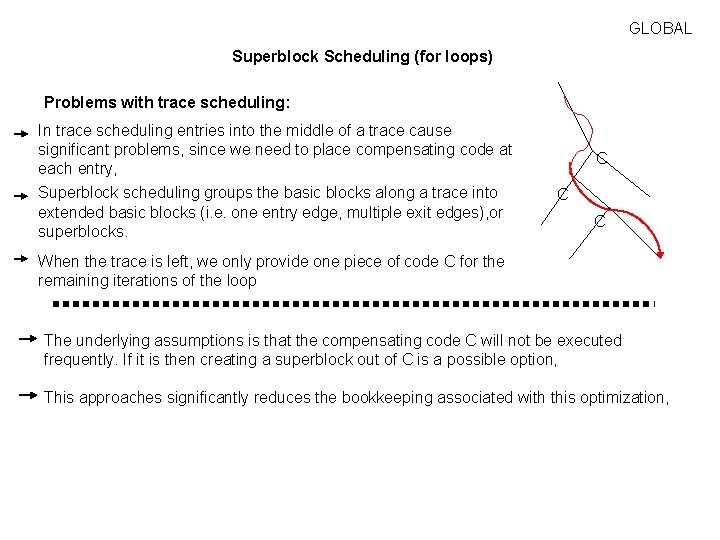
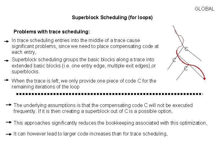
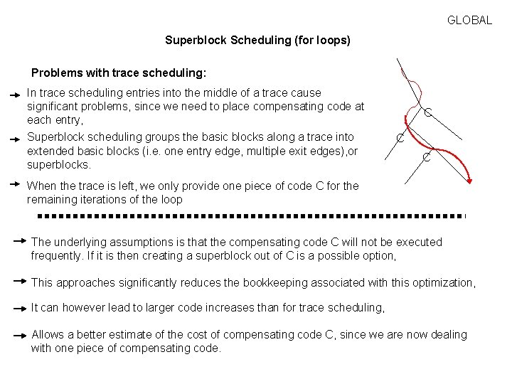
GLOBAL Superblock Scheduling (for loops) Problems with trace scheduling: In trace scheduling entries into the middle of a trace cause significant problems, since we need to place compensating code at each entry, Superblock scheduling groups the basic blocks along a trace into extended basic blocks (i. e. one entry edge, multiple exit edges), edges) or superblocks. When the trace is left, we only provide one piece of code C for the remaining iterations of the loop C C C

GLOBAL Superblock Scheduling (for loops) Problems with trace scheduling: In trace scheduling entries into the middle of a trace cause significant problems, since we need to place compensating code at each entry, Superblock scheduling groups the basic blocks along a trace into extended basic blocks (i. e. one entry edge, multiple exit edges), edges) or superblocks. C C C When the trace is left, we only provide one piece of code C for the remaining iterations of the loop The underlying assumptions is that the compensating code C will not be executed frequently. If it is then creating a superblock out of C is a possible option,

GLOBAL Superblock Scheduling (for loops) Problems with trace scheduling: In trace scheduling entries into the middle of a trace cause significant problems, since we need to place compensating code at each entry, Superblock scheduling groups the basic blocks along a trace into extended basic blocks (i. e. one entry edge, multiple exit edges), edges) or superblocks. C C C When the trace is left, we only provide one piece of code C for the remaining iterations of the loop The underlying assumptions is that the compensating code C will not be executed frequently. If it is then creating a superblock out of C is a possible option, This approaches significantly reduces the bookkeeping associated with this optimization,

GLOBAL Superblock Scheduling (for loops) Problems with trace scheduling: In trace scheduling entries into the middle of a trace cause significant problems, since we need to place compensating code at each entry, Superblock scheduling groups the basic blocks along a trace into extended basic blocks (i. e. one entry edge, multiple exit edges), edges) or superblocks. C C C When the trace is left, we only provide one piece of code C for the remaining iterations of the loop The underlying assumptions is that the compensating code C will not be executed frequently. If it is then creating a superblock out of C is a possible option, This approaches significantly reduces the bookkeeping associated with this optimization, It can however lead to larger code increases than for trace scheduling,

GLOBAL Superblock Scheduling (for loops) Problems with trace scheduling: In trace scheduling entries into the middle of a trace cause significant problems, since we need to place compensating code at each entry, Superblock scheduling groups the basic blocks along a trace into extended basic blocks (i. e. one entry edge, multiple exit edges), edges) or superblocks. C C C When the trace is left, we only provide one piece of code C for the remaining iterations of the loop The underlying assumptions is that the compensating code C will not be executed frequently. If it is then creating a superblock out of C is a possible option, This approaches significantly reduces the bookkeeping associated with this optimization, It can however lead to larger code increases than for trace scheduling, Allows a better estimate of the cost of compensating code C, since we are now dealing with one piece of compensating code.

Outline 1. Introduction 2. Basic Pipeline Scheduling 3. Instruction Level Parallelism and Dependencies 4. Local Optimizations and Loops 5. Global Scheduling Approaches 6. HW Support for Aggressive Optimization Strategies DONE DONE TALK

HW HW Support for exposing more ILP at compile-time All techniques seen so far produce potential improvements in executions time, but are subject to numerous criteria that must be satisfied, before we can safely apply these techniques,

HW HW Support for exposing more ILP at compile-time All techniques seen so far produce potential improvements in executions time, but are subject to numerous criteria that must be satisfied, before we can safely apply these techniques, If our “applicability criteria” fail, then a conservative guess is the best that we can do, so far,

HW HW Support for exposing more ILP at compile-time All techniques seen so far produce potential improvements in executions time, but are subject to numerous criteria that must be satisfied, before we can safely apply these techniques, If our “applicability criteria” fail, then a conservative guess is the best that we can do, so far, Hence we need supporting hardware mechanisms, that preserve correctness at runtime, while improving our ability to speculate effectively :

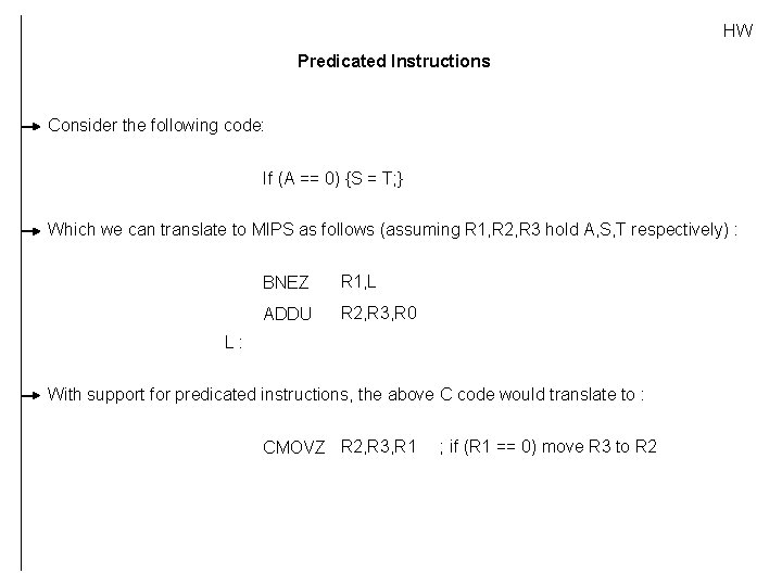
HW HW Support for exposing more ILP at compile-time All techniques seen so far produce potential improvements in executions time, but are subject to numerous criteria that must be satisfied, before we can safely apply these techniques, If our “applicability criteria” fail, then a conservative guess is the best that we can do, so far, Hence we need supporting hardware mechanisms, that preserve correctness at runtime, while improving our ability to speculate effectively : We will briefly have a look at predicated instructions, which allow us to speculate more effectively, despite the presence of control dependencies

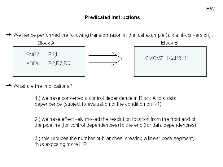
HW Predicated Instructions Consider the following code: If (A == 0) {S = T; } Which we can translate to MIPS as follows (assuming R 1, R 2, R 3 hold A, S, T respectively) : BNEZ R 1, L ADDU R 2, R 3, R 0 L: With support for predicated instructions, the above C code would translate to : CMOVZ R 2, R 3, R 1 ; if (R 1 == 0) move R 3 to R 2

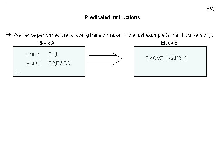
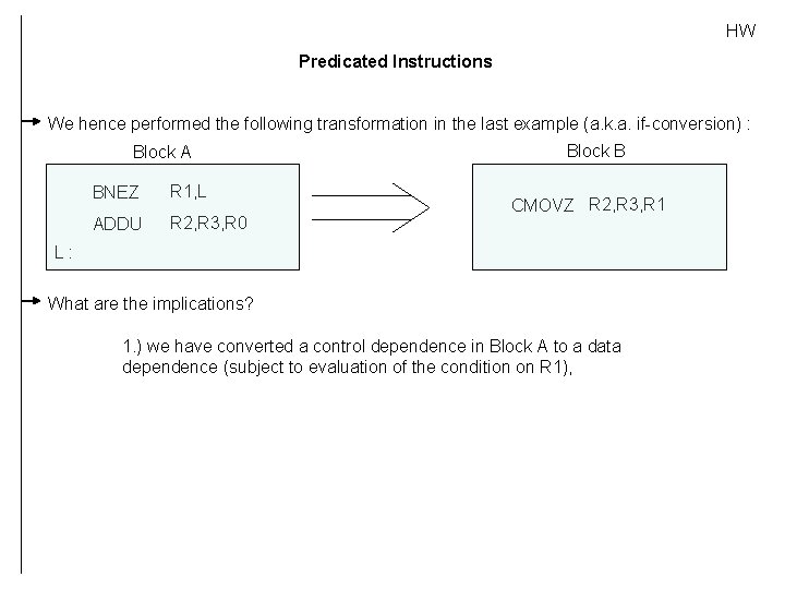
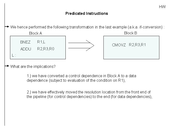
HW Predicated Instructions We hence performed the following transformation in the last example (a. k. a. if-conversion) : Block A L: BNEZ R 1, L ADDU R 2, R 3, R 0 Block B CMOVZ R 2, R 3, R 1

HW Predicated Instructions We hence performed the following transformation in the last example (a. k. a. if-conversion) : Block A BNEZ R 1, L ADDU R 2, R 3, R 0 Block B CMOVZ R 2, R 3, R 1 L: What are the implications? 1. ) we have converted a control dependence in Block A to a data dependence (subject to evaluation of the condition on R 1),

HW Predicated Instructions We hence performed the following transformation in the last example (a. k. a. if-conversion) : Block A BNEZ R 1, L ADDU R 2, R 3, R 0 Block B CMOVZ R 2, R 3, R 1 L: What are the implications? 1. ) we have converted a control dependence in Block A to a data dependence (subject to evaluation of the condition on R 1), 2. ) we have effectively moved the resolution location from the front end of the pipeline (for control dependencies) to the end (for data dependencies),

HW Predicated Instructions We hence performed the following transformation in the last example (a. k. a. if-conversion) : Block A BNEZ R 1, L ADDU R 2, R 3, R 0 Block B CMOVZ R 2, R 3, R 1 L: What are the implications? 1. ) we have converted a control dependence in Block A to a data dependence (subject to evaluation of the condition on R 1), 2. ) we have effectively moved the resolution location from the front end of the pipeline (for control dependencies) to the end (for data dependencies), 3. ) this reduces the number of branches, creating a linear code segment, thus exposing more ILP.

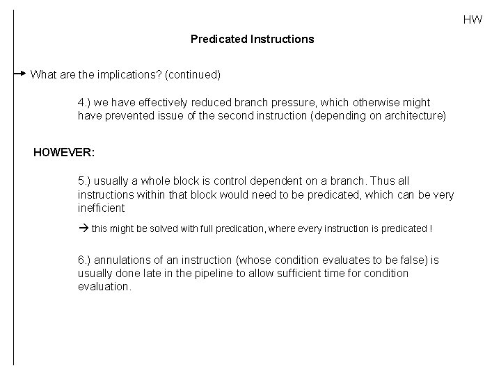
HW Predicated Instructions What are the implications? (continued) 4. ) we have effectively reduced branch pressure, which otherwise might have prevented issue of the second instruction (depending on architecture)

HW Predicated Instructions What are the implications? (continued) 4. ) we have effectively reduced branch pressure, which otherwise might have prevented issue of the second instruction (depending on architecture) HOWEVER: 5. ) usually a whole block is control dependent on a branch. Thus all instructions within that block would need to be predicated, which can be very inefficient

HW Predicated Instructions What are the implications? (continued) 4. ) we have effectively reduced branch pressure, which otherwise might have prevented issue of the second instruction (depending on architecture) HOWEVER: 5. ) usually a whole block is control dependent on a branch. Thus all instructions within that block would need to be predicated, which can be very inefficient this might be solved with full predication, where every instruction is predicated !

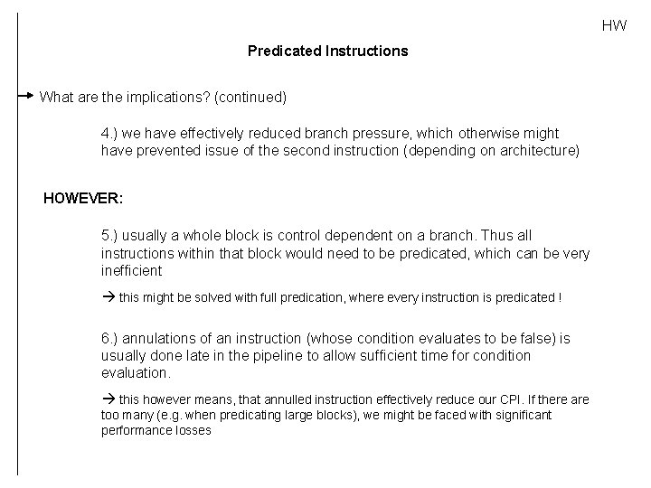
HW Predicated Instructions What are the implications? (continued) 4. ) we have effectively reduced branch pressure, which otherwise might have prevented issue of the second instruction (depending on architecture) HOWEVER: 5. ) usually a whole block is control dependent on a branch. Thus all instructions within that block would need to be predicated, which can be very inefficient this might be solved with full predication, where every instruction is predicated ! 6. ) annulations of an instruction (whose condition evaluates to be false) is usually done late in the pipeline to allow sufficient time for condition evaluation.

HW Predicated Instructions What are the implications? (continued) 4. ) we have effectively reduced branch pressure, which otherwise might have prevented issue of the second instruction (depending on architecture) HOWEVER: 5. ) usually a whole block is control dependent on a branch. Thus all instructions within that block would need to be predicated, which can be very inefficient this might be solved with full predication, where every instruction is predicated ! 6. ) annulations of an instruction (whose condition evaluates to be false) is usually done late in the pipeline to allow sufficient time for condition evaluation. this however means, that annulled instruction effectively reduce our CPI. If there are too many (e. g. when predicating large blocks), we might be faced with significant performance losses

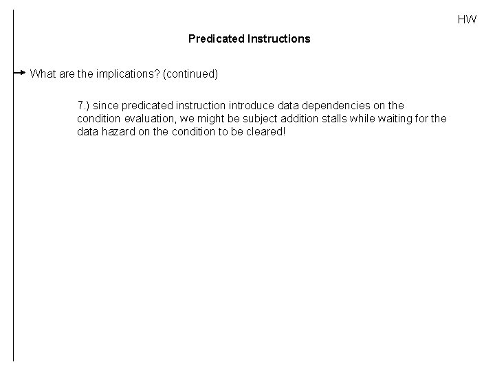
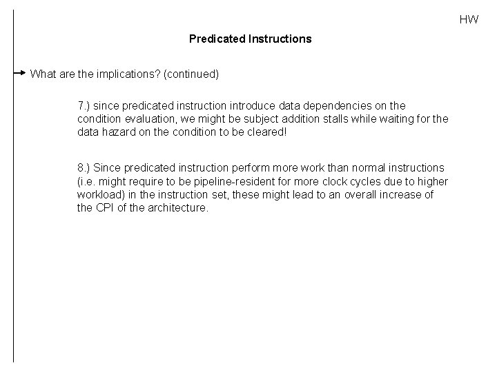
HW Predicated Instructions What are the implications? (continued) 7. ) since predicated instruction introduce data dependencies on the condition evaluation, we might be subject addition stalls while waiting for the data hazard on the condition to be cleared!

HW Predicated Instructions What are the implications? (continued) 7. ) since predicated instruction introduce data dependencies on the condition evaluation, we might be subject addition stalls while waiting for the data hazard on the condition to be cleared! 8. ) Since predicated instruction perform more work than normal instructions (i. e. might require to be pipeline-resident for more clock cycles due to higher workload) in the instruction set, these might lead to an overall increase of the CPI of the architecture.

HW Predicated Instructions What are the implications? (continued) 7. ) since predicated instruction introduce data dependencies on the condition evaluation, we might be subject addition stalls while waiting for the data hazard on the condition to be cleared! 8. ) Since predicated instruction perform more work than normal instructions (i. e. might require to be pipeline-resident for more clock cycles due to higher workload) in the instruction set, these might lead to an overall increase of the CPI of the architecture. Hence most current architectures include few simple predicated instructions

Outline 1. Introduction 2. Basic Pipeline Scheduling 3. Instruction Level Parallelism and Dependencies 4. Local Optimizations and Loops 5. Global Scheduling Approaches 6. HW Support for Aggressive Optimization Strategies Just a brief summary to go! DONE DONE

SUM SUMMARY 1. ) Compile-Time optimizations provide a number of analysis-intensive optimizations that otherwise could not be performed at run-time due to the high overhead associated with the analysis.

SUM SUMMARY 1. ) Compile-Time optimizations provide a number of analysis-intensive optimizations that otherwise could not be performed at run-time due to the high overhead associated with the analysis. 2. ) Compiler based approaches are usually limited by the inaccuracy or unavailability of data and control flow behavioral information of the program at run time.

SUM SUMMARY 1. ) Compile-Time optimizations provide a number of analysis-intensive optimizations that otherwise could not be performed at run-time due to the high overhead associated with the analysis. 2. ) Compiler based approaches are usually limited by the inaccuracy or unavailability of data and control flow behavioral information of the program at run time. 3. ) Compilers can reorganize code such that more ILP is exposed for further optimizations or more ILP during run-time.

SUM SUMMARY 1. ) Compile-Time optimizations provide a number of analysis-intensive optimizations that otherwise could not be performed at run-time due to the high overhead associated with the analysis. 2. ) Compiler based approaches are usually limited by the inaccuracy or unavailability of data and control flow behavioral information of the program at run time. 3. ) Compilers can reorganize code such that more ILP is exposed for further optimizations or more ILP during run-time. CONCLUSION: 1. ) The most efficient approach is a hardware software co-scheduling approach, where the hardware and compiler co-operatively exploit as much information as possible within the respective restrictions of each approach. 2. ) Such an approach is most likely to produce highest performance!

REF REFERENCES 1. “Computer Architecture: A Quantitative Approach”. J. L. Hennessy & D. A. Patterson. Morgan Kaufmann Publishers, 3 rd Edition. 2. “Optimizing Compilers for Modern Architectures”. S. Muchnik. Morgan Kaufmann Publishers, 2 nd Edition. 3. “Advanced Compiler Design & Implementation”. S. Muchnik. Morgan Kaufmann Publishers, 2 nd Edition. 4. “Compilers: Principles, Techniques and Tools”: A. V. Aho, R. Sethi, J. D. Ullman. Addision Wesly Longman Publishers, 2 nd Edition.