Chapter 9 Algorithm Efficiency and Sorting Chien Chin

Chapter 9: Algorithm Efficiency and Sorting Chien Chin Chen Department of Information Management National Taiwan University

Measuring the Efficiency of Algorithms (1/5) o Measuring an algorithm’s efficiency is very important. n o Your choice of algorithm for a application often has a great impact. Components that contribute to the cost of a computer program: n The cost of human time. o n Time of development, maintenance … The cost of program execution. o The amount of computer time and space that the program requires to execute. 2

Measuring the Efficiency of Algorithms (2/5) o Analysis of algorithms: n Provides tools for contrasting the efficiency of different algorithms. o n n Time efficiency, space efficiency Should focus on significant differences in efficiency. Should not consider reductions in computing costs due to clever coding tricks. 3

Measuring the Efficiency of Algorithms (3/5) o o o This chapter focuses on time efficiency. Comparison: implement different programs; check which one is faster. Three difficulties with comparing programs instead of algorithms: n n n How are the algorithms coded? What computer should you use? What data should the programs use? o The most important difficulty. 4

Measuring the Efficiency of Algorithms (4/5) o Algorithm analysis should be independent of : n n n o Specific implementations. Computers. Data. How? n Counting the number of significant operations in a particular solution. 5

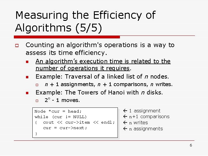
Measuring the Efficiency of Algorithms (5/5) o Counting an algorithm's operations is a way to assess its time efficiency. n n An algorithm’s execution time is related to the number of operations it requires. Example: Traversal of a linked list of n nodes. o n n + 1 assignments, n + 1 comparisons, n writes. Example: The Towers of Hanoi with n disks. o 2 n - 1 moves. Node *cur = head; while (cur != NULL) { cout << cur->item << endl; cur = cur->next; } 1 assignment n+1 comparisons n writes n assignments 6

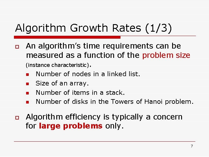
Algorithm Growth Rates (1/3) o An algorithm’s time requirements can be measured as a function of the problem size (instance characteristic). n n o Number of nodes in a linked list. Size of an array. Number of items in a stack. Number of disks in the Towers of Hanoi problem. Algorithm efficiency is typically a concern for large problems only. 7

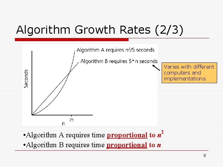
Algorithm Growth Rates (2/3) Varies with different computers and implementations. • Algorithm A requires time proportional to n 2 • Algorithm B requires time proportional to n 8

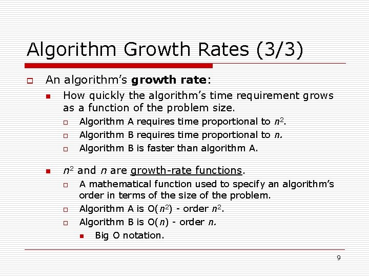
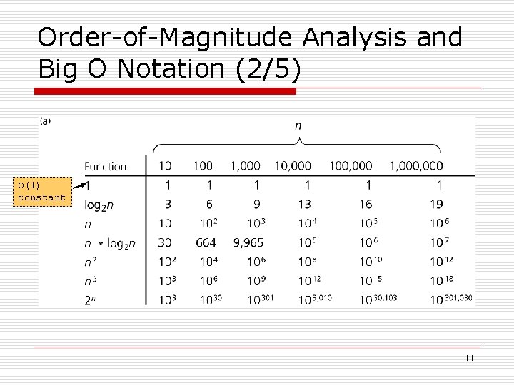
Algorithm Growth Rates (3/3) o An algorithm’s growth rate: n How quickly the algorithm’s time requirement grows as a function of the problem size. o o o n Algorithm A requires time proportional to n 2. Algorithm B requires time proportional to n. Algorithm B is faster than algorithm A. n 2 and n are growth-rate functions. o o o A mathematical function used to specify an algorithm’s order in terms of the size of the problem. Algorithm A is O(n 2) - order n 2. Algorithm B is O(n) - order n. n Big O notation. 9

Order-of-Magnitude Analysis and Big O Notation (1/5) o Definition of the order of an algorithm: Algorithm A is order f(n) – denoted O (f(n)) – if constants k and n 0 exist such that A requires no more than k * f(n) time units to solve a problem of size n ≥ n 0. 10

Order-of-Magnitude Analysis and Big O Notation (2/5) O(1) constant 11

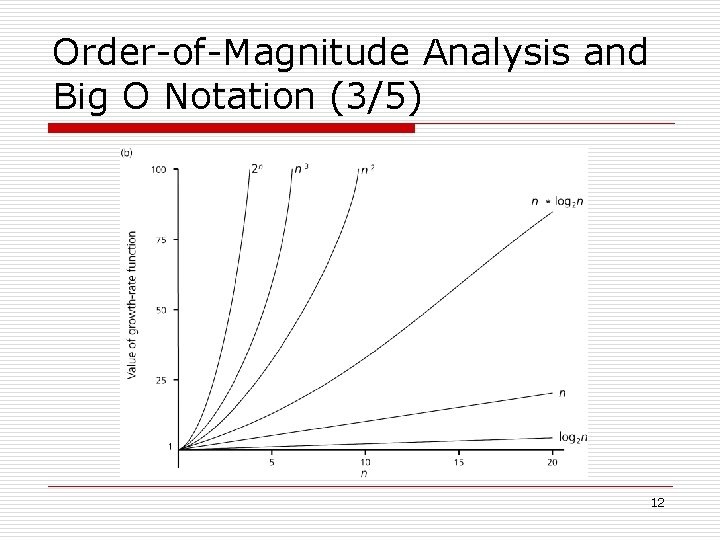
Order-of-Magnitude Analysis and Big O Notation (3/5) 12

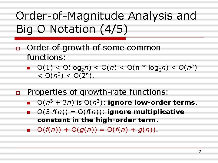
Order-of-Magnitude Analysis and Big O Notation (4/5) o Order of growth of some common functions: n o O(1) < O(log 2 n) < O(n * log 2 n) < O(n 2) < O(n 3) < O(2 n). Properties of growth-rate functions: n n n O(n 3 + 3 n) is O(n 3): ignore low-order terms. O(5 f(n)) = O(f(n)): ignore multiplicative constant in the high-order term. O(f(n)) + O(g(n)) = O(f(n) + g(n)). 13

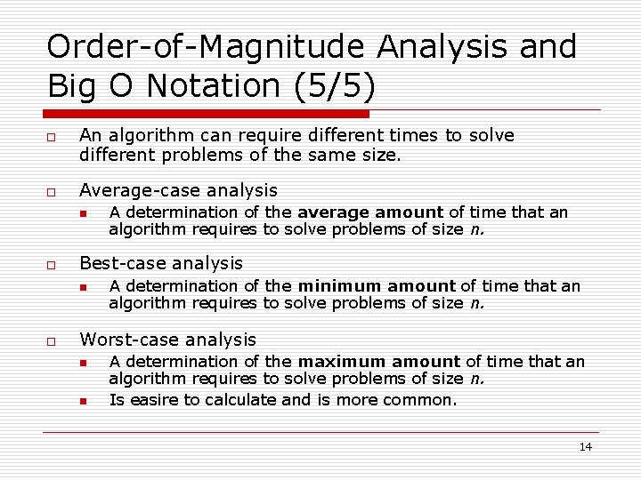
Order-of-Magnitude Analysis and Big O Notation (5/5) o o An algorithm can require different times to solve different problems of the same size. Average-case analysis n o Best-case analysis n o A determination of the average amount of time that an algorithm requires to solve problems of size n. A determination of the minimum amount of time that an algorithm requires to solve problems of size n. Worst-case analysis n n A determination of the maximum amount of time that an algorithm requires to solve problems of size n. Is easire to calculate and is more common. 14

Keeping Your Perspective (1/2) o o Only significant differences in efficiency are interesting. Frequency of operations: n n When choosing an ADT’s implementation, consider how frequently particular ADT operations occur in a given application. However, some seldom-used but critical operations must be efficient. o E. g. , an air traffic control system. 15

Keeping Your Perspective (2/2) o If the problem size is always small, you can probably ignore an algorithm’s efficiency. n o o Order-of-magnitude analysis focuses on large problems. Weigh the trade-offs between an algorithm’s time requirements and its memory requirements. Compare algorithms for both style and efficiency. 16

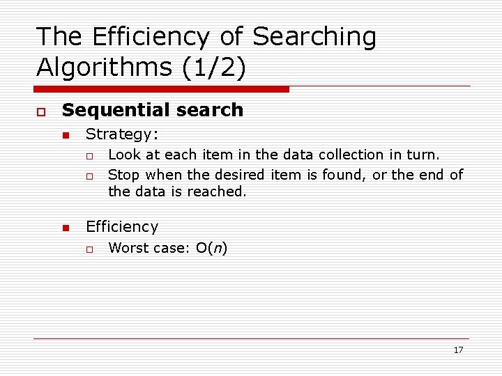
The Efficiency of Searching Algorithms (1/2) o Sequential search n Strategy: o o n Look at each item in the data collection in turn. Stop when the desired item is found, or the end of the data is reached. Efficiency o Worst case: O(n) 17

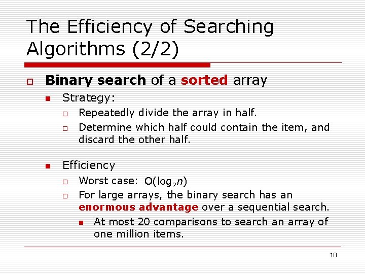
The Efficiency of Searching Algorithms (2/2) o Binary search of a sorted array n Strategy: o o n Repeatedly divide the array in half. Determine which half could contain the item, and discard the other half. Efficiency o o Worst case: O(log 2 n) For large arrays, the binary search has an enormous advantage over a sequential search. n At most 20 comparisons to search an array of one million items. 18

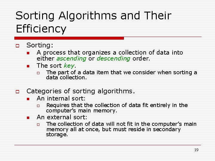
Sorting Algorithms and Their Efficiency o Sorting: n n A process that organizes a collection of data into either ascending or descending order. The sort key. o o The part of a data item that we consider when sorting a data collection. Categories of sorting algorithms. n An internal sort: o n Requires that the collection of data fit entirely in the computer’s main memory. An external sort: o The collection of data will not fit in the computer’s main memory all at once, but must reside in secondary storage. 19

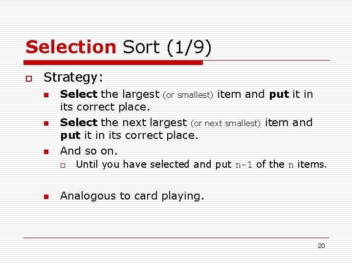
Selection Sort (1/9) o Strategy: n n n Select the largest (or smallest) item and put it in its correct place. Select the next largest (or next smallest) item and put it in its correct place. And so on. o n Until you have selected and put n-1 of the n items. Analogous to card playing. 20

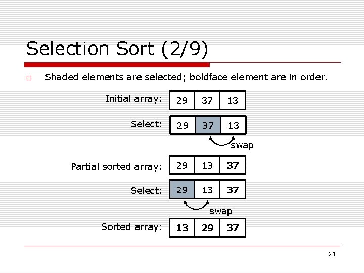
Selection Sort (2/9) o Shaded elements are selected; boldface element are in order. Initial array: 29 37 13 Select: 29 37 13 swap Partial sorted array: 29 13 37 Select: 29 13 37 swap Sorted array: 13 29 37 21

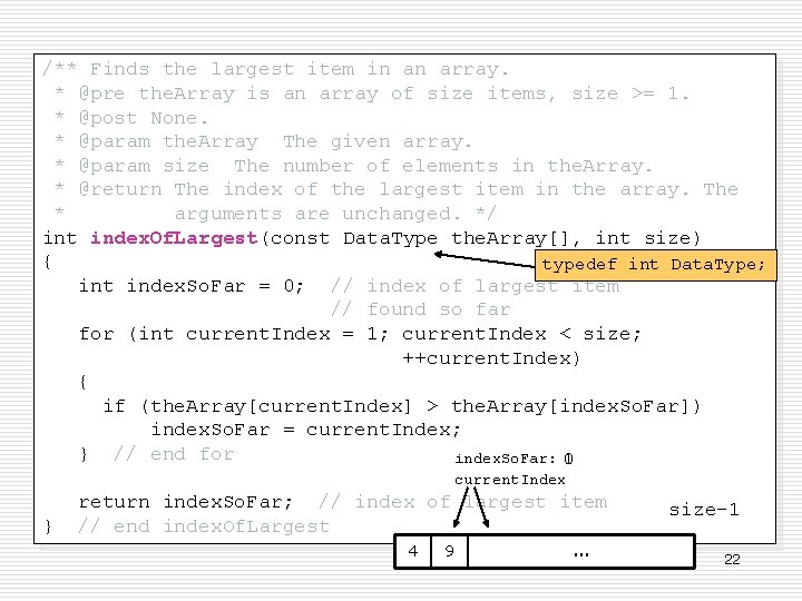
/** Finds the largest item in an array. * @pre the. Array is an array of size items, size >= 1. * @post None. * @param the. Array The given array. * @param size The number of elements in the. Array. * @return The index of the largest item in the array. The * arguments are unchanged. */ int index. Of. Largest(const Data. Type the. Array[], int size) { typedef int Data. Type; int index. So. Far = 0; // index of largest item // found so far for (int current. Index = 1; current. Index < size; ++current. Index) { if (the. Array[current. Index] > the. Array[index. So. Far]) index. So. Far = current. Index; } // end for index. So. Far: 0 1 current. Index } return index. So. Far; // index of largest item // end index. Of. Largest 4 9 . . . size-1 22

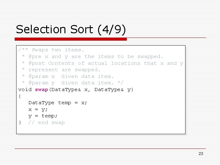
Selection Sort (4/9) /** Swaps two items. * @pre x and y are the items to be swapped. * @post Contents of actual locations that x and y * represent are swapped. * @param x Given data item. * @param y Given data item. */ void swap(Data. Type& x, Data. Type& y) { Data. Type temp = x; x = y; y = temp; } // end swap 23

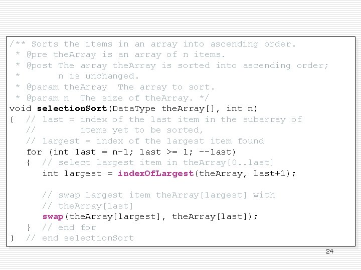
Selection Sort (5/) /** Sorts the items in an array into ascending order. * @pre the. Array is an array of n items. * @post The array the. Array is sorted into ascending order; * n is unchanged. * @param the. Array The array to sort. * @param n The size of the. Array. */ void selection. Sort(Data. Type the. Array[], int n) { // last = index of the last item in the subarray of // items yet to be sorted, // largest = index of the largest item found for (int last = n-1; last >= 1; --last) { // select largest item in the. Array[0. . last] int largest = index. Of. Largest(the. Array, last+1); } // swap largest item the. Array[largest] with // the. Array[last] swap(the. Array[largest], the. Array[last]); } // end for // end selection. Sort 24

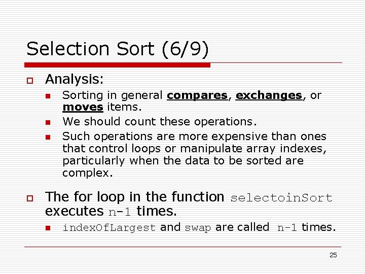
Selection Sort (6/9) o Analysis: n n n o Sorting in general compares, exchanges, or moves items. We should count these operations. Such operations are more expensive than ones that control loops or manipulate array indexes, particularly when the data to be sorted are complex. The for loop in the function selectoin. Sort executes n-1 times. n index. Of. Largest and swap are called n-1 times. 25

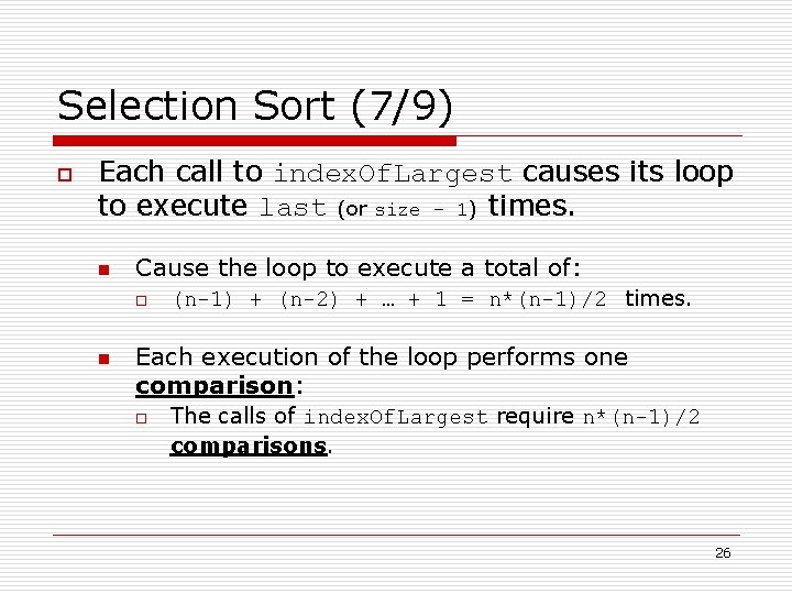
Selection Sort (7/9) o Each call to index. Of. Largest causes its loop to execute last (or size – 1) times. n Cause the loop to execute a total of: o n (n-1) + (n-2) + … + 1 = n*(n-1)/2 times. Each execution of the loop performs one comparison: o The calls of index. Of. Largest require n*(n-1)/2 comparisons. 26

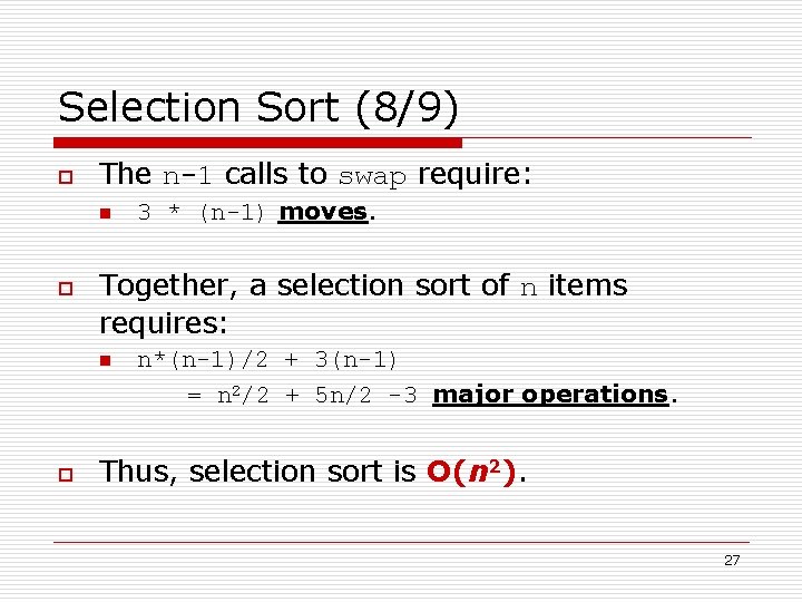
Selection Sort (8/9) o The n-1 calls to swap require: n o Together, a selection sort of n items requires: n o 3 * (n-1) moves. n*(n-1)/2 + 3(n-1) = n 2/2 + 5 n/2 -3 major operations. Thus, selection sort is O(n 2). 27

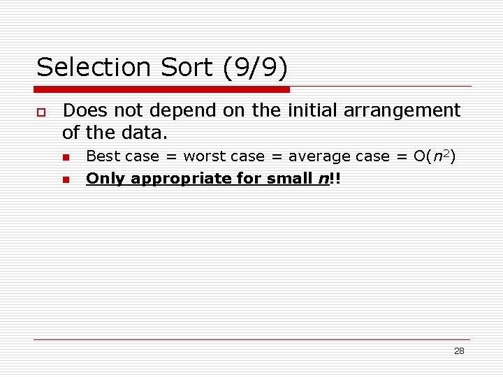
Selection Sort (9/9) o Does not depend on the initial arrangement of the data. n n Best case = worst case = average case = O(n 2) Only appropriate for small n!! 28

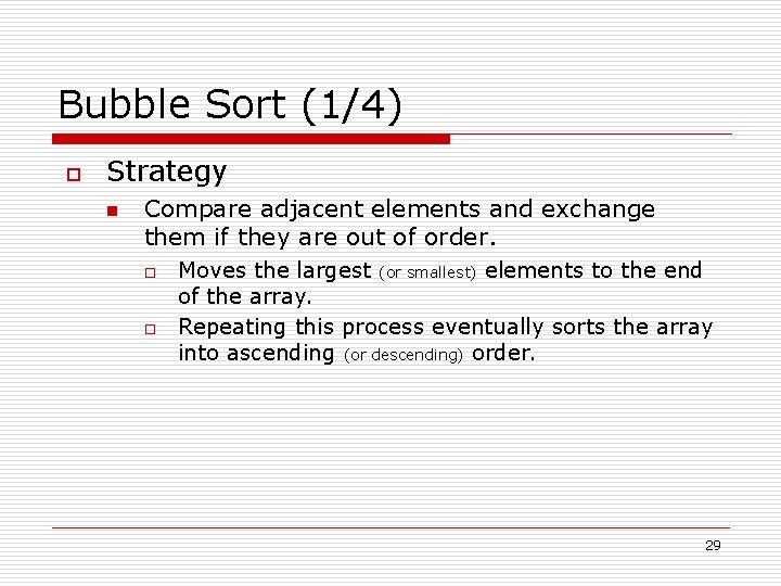
Bubble Sort (1/4) o Strategy n Compare adjacent elements and exchange them if they are out of order. o o Moves the largest (or smallest) elements to the end of the array. Repeating this process eventually sorts the array into ascending (or descending) order. 29

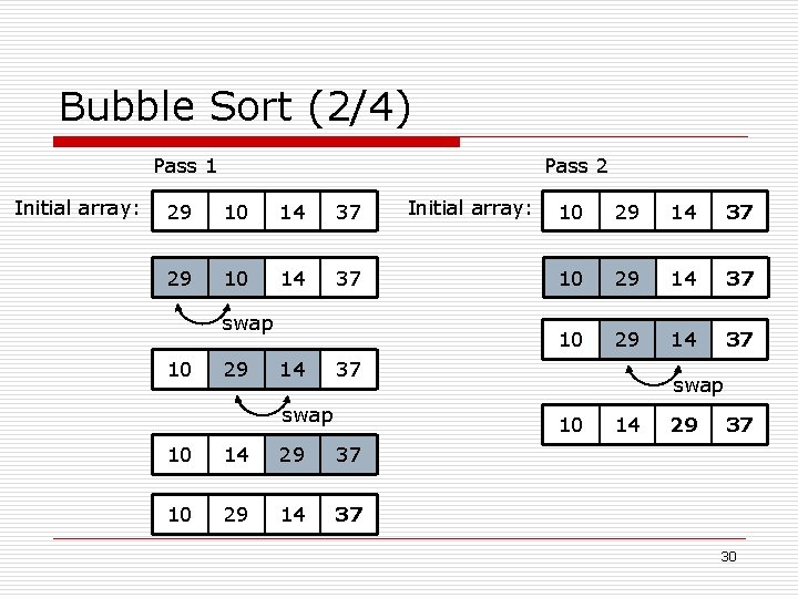
Bubble Sort (2/4) Pass 1 Initial array: Pass 2 29 10 14 37 swap 10 29 14 Initial array: 10 29 14 37 37 swap 10 10 14 29 37 10 29 14 37 14 29 37 30

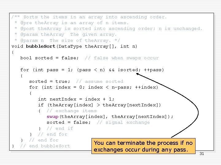
/** Sorts the items in an array into ascending order. * @pre the. Array is an array of n items. * @post the. Array is sorted into ascending order; n is unchanged. * @param the. Array The given array. * @param n The size of the. Array. */ void bubble. Sort(Data. Type the. Array[], int n) { bool sorted = false; // false when swaps occur Bubble Sort (3/) } for (int pass = 1; (pass < n) && !sorted; ++pass) { sorted = true; // assume sorted for (int index = 0; index < n-pass; ++index) { int next. Index = index + 1; if (the. Array[index] > the. Array[next. Index]) { // exchange items swap(the. Array[index], the. Array[next. Index]); sorted = false; // signal exchange } // end if } // end for You can terminate the process if no // end bubble. Sort exchanges occur during any pass. 31

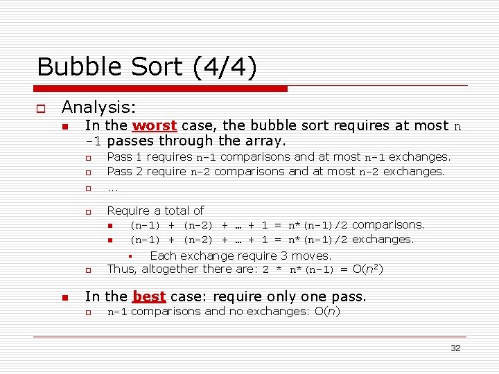
Bubble Sort (4/4) o Analysis: n In the worst case, the bubble sort requires at most n -1 passes through the array. o o o n Pass 1 requires n-1 comparisons and at most n-1 exchanges. Pass 2 require n-2 comparisons and at most n-2 exchanges. . Require a total of n (n-1) + (n-2) + … + 1 = n*(n-1)/2 comparisons. n (n-1) + (n-2) + … + 1 = n*(n-1)/2 exchanges. § Each exchange require 3 moves. Thus, altogethere are: 2 * n*(n-1) = O(n 2) In the best case: require only one pass. o n-1 comparisons and no exchanges: O(n) 32

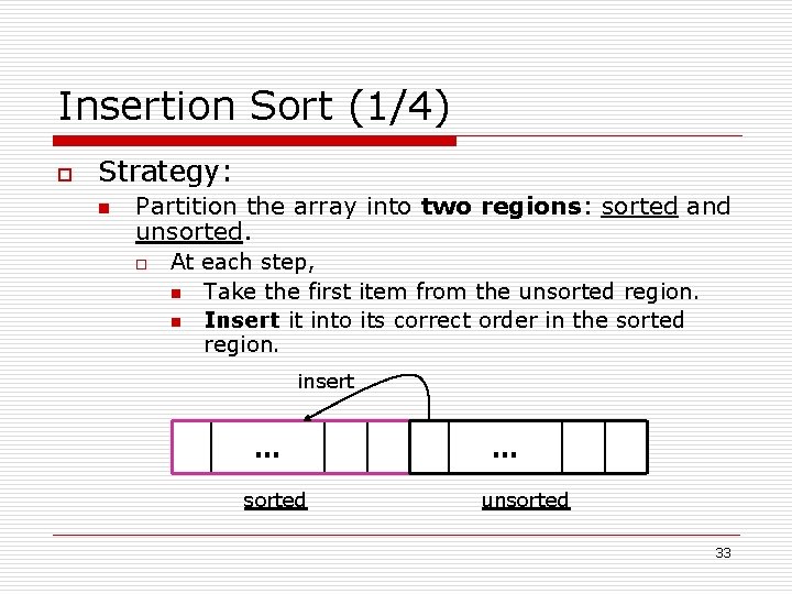
Insertion Sort (1/4) o Strategy: n Partition the array into two regions: sorted and unsorted. o At each step, n Take the first item from the unsorted region. n Insert it into its correct order in the sorted region. insert … sorted … unsorted 33

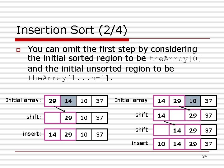
Insertion Sort (2/4) o You can omit the first step by considering the initial sorted region to be the. Array[0] and the initial unsorted region to be the. Array[1. . . n-1]. Initial array: 29 shift: insert: 14 14 10 37 29 10 37 Initial array: 14 shift: insert: 10 29 10 37 29 37 14 29 37 34

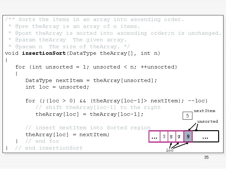
/** Sorts the items in an array into ascending order. * @pre the. Array is an array of n items. * @post the. Array is sorted into ascending order; n is unchanged. * @param the. Array The given array. * @param n The size of the. Array. */ void insertion. Sort(Data. Type the. Array[], int n) { for (int unsorted = 1; unsorted < n; ++unsorted) { Data. Type next. Item = the. Array[unsorted]; int loc = unsorted; Insertion Sort (3/) for (; (loc > 0) && (the. Array[loc-1]> next. Item); --loc) // shift the. Array[loc-1] to the right next. Item the. Array[loc] = the. Array[loc-1]; 5 unsorted } // insert next. Item into Sorted region the. Array[loc] = next. Item; . . . } // end for // end insertion. Sort 3 5 7 7 9 9 5 . . . loc 35

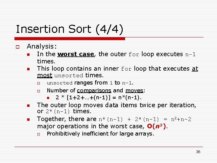
Insertion Sort (4/4) o Analysis: n n In the worst case, the outer for loop executes n-1 times. This loop contains an inner for loop that executes at most unsorted times. o o n n unsorted ranges from 1 to n-1. Number of comparisons and moves: n 2 * [1+2+…+(n-1)] = n*(n-1). The outer loop moves data items twice per iteration, or 2*(n-1) times. Together, there are n*(n-1) + 2*(n-1) = n 2+n-2 major operations in the worst case, O(n 2). o Prohibitively inefficient for large arrays. 36

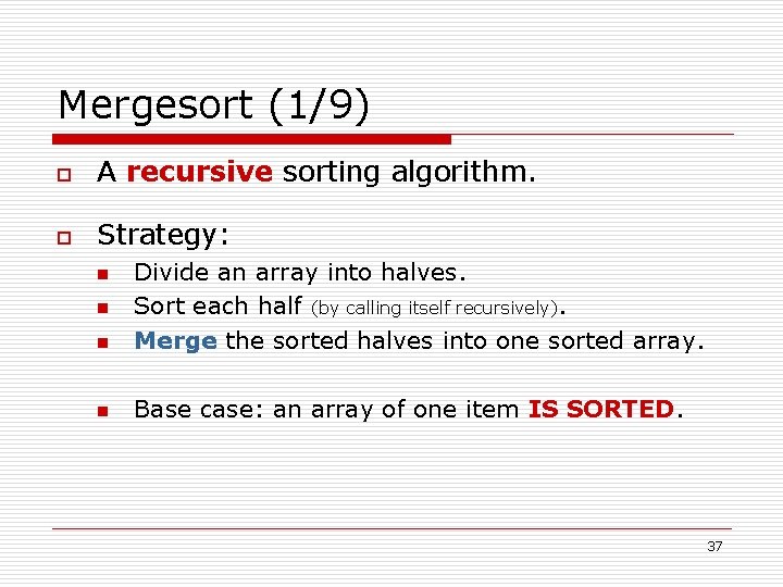
Mergesort (1/9) o A recursive sorting algorithm. o Strategy: n Divide an array into halves. Sort each half (by calling itself recursively). Merge the sorted halves into one sorted array. n Base case: an array of one item IS SORTED. n n 37

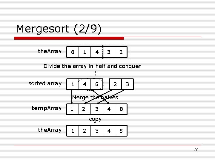
Mergesort (2/9) the. Array: 8 1 4 3 2 Divide the array in half and conquer. . . sorted array: 1 4 8 2 3 Merge the halves temp. Array: 1 2 3 4 8 copy the. Array: 1 2 3 38

Mergesort (3/9) /** Sorts the items in an array into ascending order. * @pre the. Array[first. . last] is an array. * @post the. Array[first. . last] is sorted in ascending order. * @param the. Array The given array. * @param first The first element to consider in the. Array. * @param last The last element to consider in the. Array. */ void mergesort(Data. Type the. Array[], int first, int last) { if (first < last) { int mid = (first + last)/2; // index of midpoint mergesort(the. Array, first, mid); mergesort(the. Array, mid+1, last); } // merge the two halves merge(the. Array, first, mid, last); } // end if // end mergesort 39

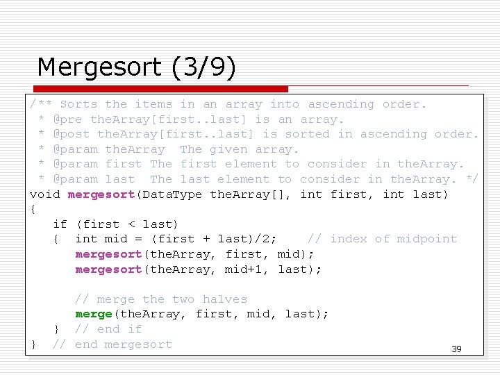
const int MAX_SIZE = 10000; void merge(Data. Type the. Array[], int first, int mid, int last) { Data. Type temp. Array[MAX_SIZE]; // temporary array Mergesort (4/) // initialize the local indexes to indicate the subarrays int first 1 = first; // beginning of first subarray int last 1 = mid; // end of first subarray int first 2 = mid + 1; // beginning of second subarray int last 2 = last; // end of second subarray // while both subarrays are not empty, copy the // smaller item into the temporary array int index = first 1; // next available location in // temp. Array for (; (first 1 <= last 1) && (first 2 <= last 2); ++index) { if (the. Array[first 1] < the. Array[first 2]) first 1 last 1 first 2 { temp. Array[index] = the. Array[first 1]; ++first 1; … 3 9 an. Array. . . 5 8 } else first mid { temp. Array[index] = the. Array[first 2]; index ++first 2; } // end if. . . 3 5. . . temp. Array } // end for last 2. . . last 40 . . .

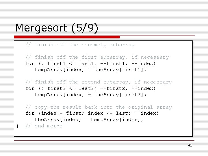
Mergesort (5/9) // finish off the nonempty subarray // finish off the first subarray, if necessary for (; first 1 <= last 1; ++first 1, ++index) temp. Array[index] = the. Array[first 1]; // finish off the second subarray, if necessary for (; first 2 <= last 2; ++first 2, ++index) temp. Array[index] = the. Array[first 2]; } // copy the result back into the original array for (index = first; index <= last; ++index) the. Array[index] = temp. Array[index]; // end merge 41

Mergesort (6/9) void mergesort(Data. Type the. Array[], int first, int last) { if (first < last) { int mid = (first + last)/2; mergesort(the. Array, first, mid); mergesort(the. Array, mid+1, last); merge(the. Array, first, mid, last); } mergesort(the. Array, 0, 5) } mergesort(the. Array, 0, 2) mergesort(the. Array, 3, 5) mergesort(the. Array, 0, 1) mergesort(the. Array, 1, 1) 42

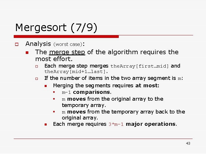
Mergesort (7/9) o Analysis (worst case): n The merge step of the algorithm requires the most effort. o o Each merge step merges the. Array[first…mid] and the. Array[mid+1…last]. If the number of items in the two array segment is m: n Merging the segments requires at most: § m-1 comparisons. § m moves from the original array to the temporary array. § m moves from the temporary array back to the original array. n Each merge requires 3*m-1 major operations. 43

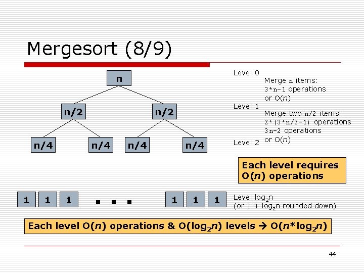
Mergesort (8/9) Level 0 n n/2 n/4 Level 1 n/2 n/4 Merge n items: 3*n-1 operations or O(n) Merge two n/2 items: 2*(3*n/2 -1) operations 3 n-2 operations Level 2 or O(n) n/4 Each level requires O(n) operations 1 1 1 . . . 1 1 1 Level log 2 n (or 1 + log 2 n rounded down) Each level O(n) operations & O(log 2 n) levels O(n*log 2 n) 44

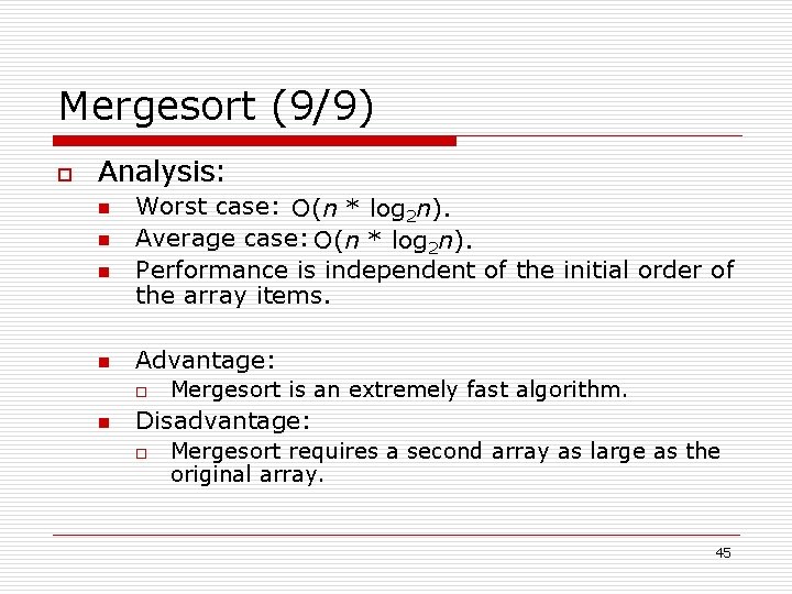
Mergesort (9/9) o Analysis: n n Worst case: O(n * log 2 n). Average case: O(n * log 2 n). Performance is independent of the initial order of the array items. Advantage: o n Mergesort is an extremely fast algorithm. Disadvantage: o Mergesort requires a second array as large as the original array. 45

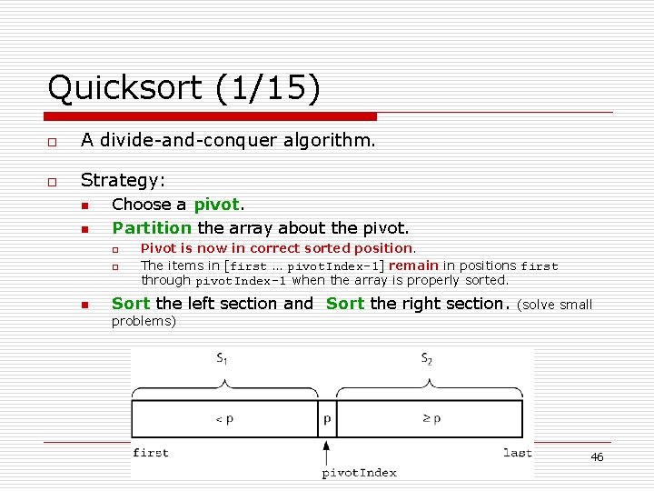
Quicksort (1/15) o A divide-and-conquer algorithm. o Strategy: n n Choose a pivot. Partition the array about the pivot. o o n Pivot is now in correct sorted position. The items in [first … pivot. Index-1] remain in positions first through pivot. Index-1 when the array is properly sorted. Sort the left section and Sort the right section. (solve small problems) 46

Quicksort (2/15) o Partition algorithm: n To partition an array segment the. Array[first…last]. n Choose a pivot. o o n If the items in the array are arranged randomly, you can choose a pivot at random. Choose the. Array[first] as the pivot. Three regions: S 1, S 2, and unknown. 47

Quicksort (3/15) n Initially, all items except the pivot (the. Array[first]) constitute the unknown region. o Conditions: n last. S 1 = first n first. Unknown = first + 1 p ? first. Unknown last. S 1 n At each stop, you examine one item of the unknown region. o n n last i. e. , the. Array[first. Unknown]. Determine in which of the S 1 or S 2 it belongs, and place it there. Then decrease the size of unknown by 1 (i. e. , first. Unknown++). 48

Quicksort (4/15) n Move the. Array[first. Unknown] into S 1: o o o Swap the. Array[first. Unknown] with the. Array[last. S 1+1]. Increment last. S 1. Increment first. Unknown. swap S 2 S 1 p first <p ≧p <p last. S 1 ≧p unknown <p ≧p ? first. Unknown last 49

Quicksort (5/15) n Move the. Array[first. Unknown] into S 2: o Simply increment first. Unknown by 1. S 2 S 1 p first <p ≧p last. S 1 unknown ≧p ? first. Unknown last 50

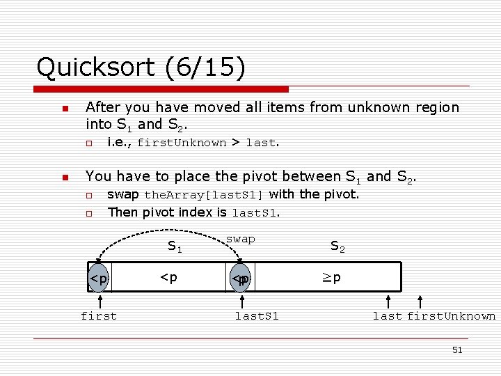
Quicksort (6/15) n After you have moved all items from unknown region into S 1 and S 2. o n i. e. , first. Unknown > last. You have to place the pivot between S 1 and S 2. o o swap the. Array[last. S 1] with the pivot. Then pivot index is last. S 1 p <p first <p swap <p p last. S 1 S 2 ≧p last first. Unknown 51

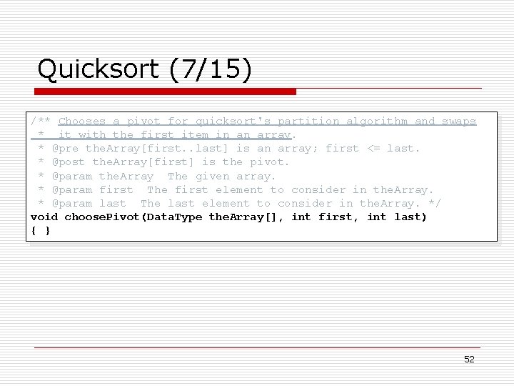
Quicksort (7/15) /** Chooses a pivot for quicksort's partition algorithm and swaps * it with the first item in an array. * @pre the. Array[first. . last] is an array; first <= last. * @post the. Array[first] is the pivot. * @param the. Array The given array. * @param first The first element to consider in the. Array. * @param last The last element to consider in the. Array. */ void choose. Pivot(Data. Type the. Array[], int first, int last) { } 52

Quicksort (8/15) void partition(Data. Type the. Array[], int first, int last, int& pivot. Index) { // place pivot in the. Array[first] choose. Pivot(the. Array, first, last); Data. Type pivot = the. Array[first]; // copy pivot // initially, everything but pivot is in unknown int last. S 1 = first; // index of last item in S 1 int first. Unknown = first + 1; // index of first item in // unknown p first. Unknown last. S 1 ? last 53

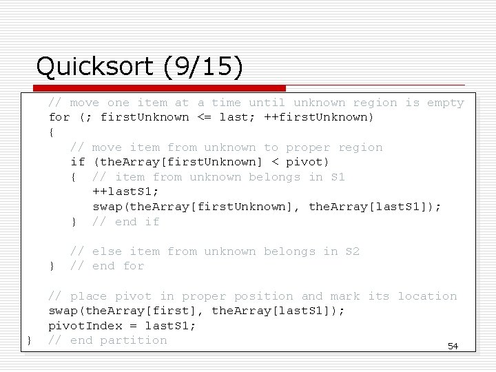
Quicksort (9/15) // move one item at a time until unknown region is empty for (; first. Unknown <= last; ++first. Unknown) { // move item from unknown to proper region if (the. Array[first. Unknown] < pivot) { // item from unknown belongs in S 1 ++last. S 1; swap(the. Array[first. Unknown], the. Array[last. S 1]); } // end if } } // else item from unknown belongs in S 2 // end for // place pivot in proper position and mark its location swap(the. Array[first], the. Array[last. S 1]); pivot. Index = last. S 1; // end partition 54

Quicksort (10/15) void quicksort(Data. Type the. Array[], int first, int last) { int pivot. Index; if (first < last) { // create the partition: S 1, pivot, S 2 partition(the. Array, first, last, pivot. Index); } // sort regions S 1 and S 2 quicksort(the. Array, first, pivot. Index-1); quicksort(the. Array, pivot. Index+1, last); } // end if // end quicksort 55

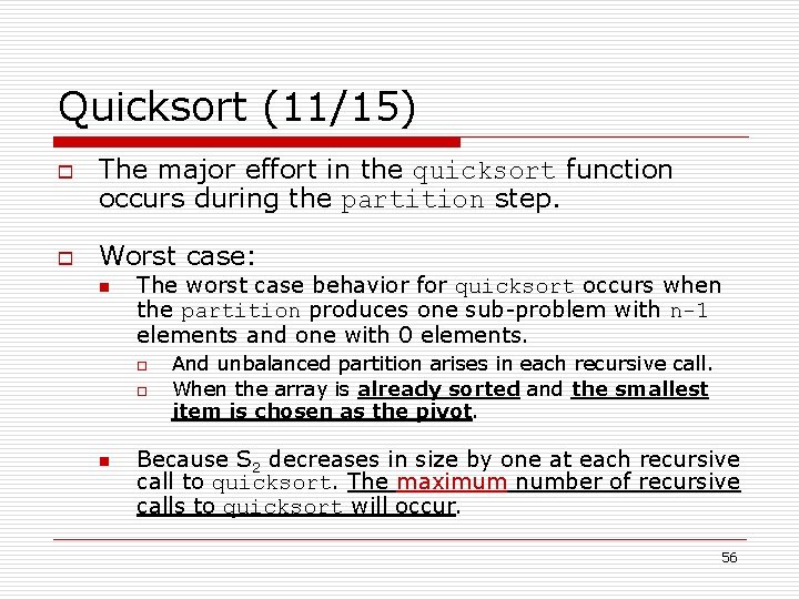
Quicksort (11/15) o o The major effort in the quicksort function occurs during the partition step. Worst case: n The worst case behavior for quicksort occurs when the partition produces one sub-problem with n-1 elements and one with 0 elements. o o n And unbalanced partition arises in each recursive call. When the array is already sorted and the smallest item is chosen as the pivot. Because S 2 decreases in size by one at each recursive call to quicksort. The maximum number of recursive calls to quicksort will occur. 56

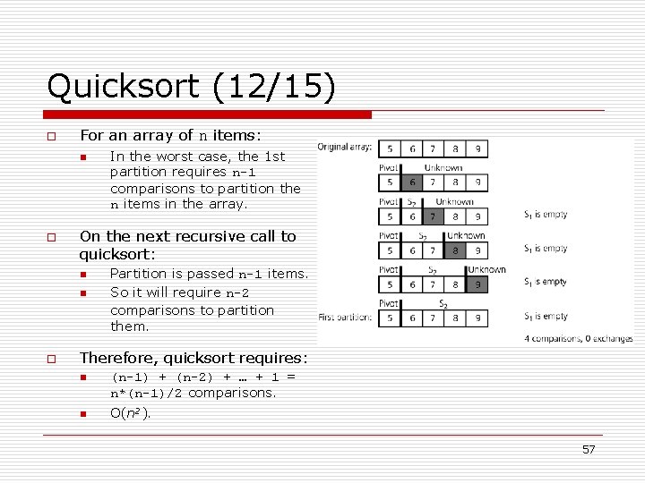
Quicksort (12/15) o For an array of n items: n o On the next recursive call to quicksort: n n o In the worst case, the 1 st partition requires n-1 comparisons to partition the n items in the array. Partition is passed n-1 items. So it will require n-2 comparisons to partition them. Therefore, quicksort requires: n n (n-1) + (n-2) + … + 1 = n*(n-1)/2 comparisons. O(n 2). 57

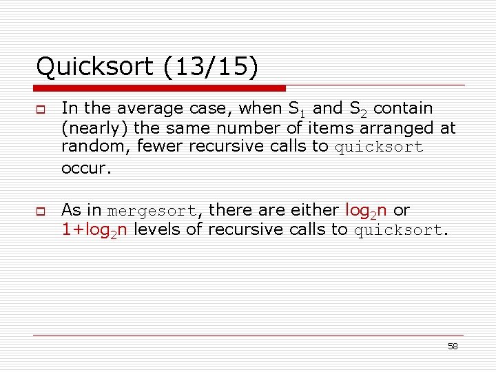
Quicksort (13/15) o o In the average case, when S 1 and S 2 contain (nearly) the same number of items arranged at random, fewer recursive calls to quicksort occur. As in mergesort, there are either log 2 n or 1+log 2 n levels of recursive calls to quicksort. 58

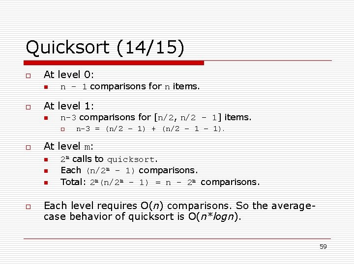
Quicksort (14/15) o At level 0: n o n – 1 comparisons for n items. At level 1: n n-3 comparisons for [n/2, n/2 – 1] items. o o At level m: n n n o n-3 = (n/2 – 1) + (n/2 – 1). 2 m calls to quicksort. Each (n/2 m – 1) comparisons. Total: 2 m(n/2 m – 1) = n – 2 m comparisons. Each level requires O(n) comparisons. So the averagecase behavior of quicksort is O(n*logn). 59

Quicksort (15/15) n n Quicksort is usually extremely fast in practice. Even if the worst case occurs, quicksort’s performance is acceptable for moderately large arrays. 60

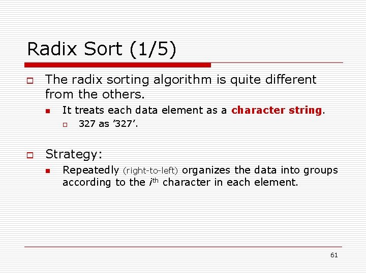
Radix Sort (1/5) o The radix sorting algorithm is quite different from the others. n It treats each data element as a character string. o o 327 as ’ 327’. Strategy: n Repeatedly (right-to-left) organizes the data into groups according to the ith character in each element. 61

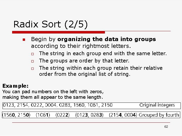
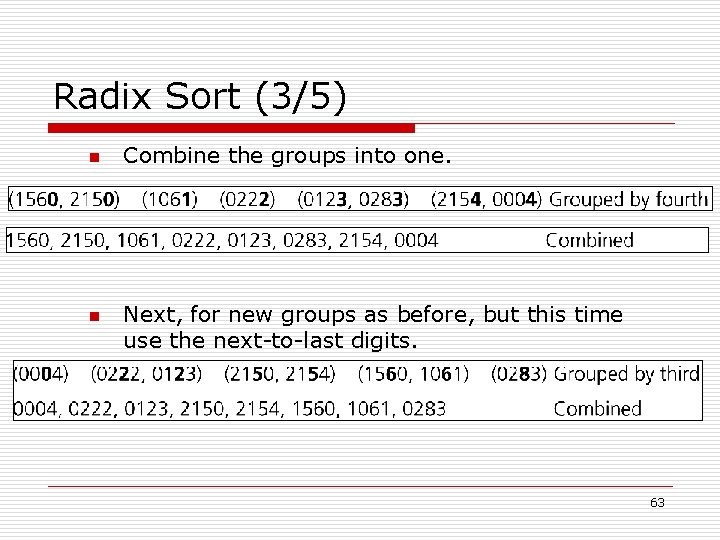
Radix Sort (2/5) n Begin by organizing the data into groups according to their rightmost letters. o o o The string in each group end with the same letter. The groups are order by that letter. The string within each group retain their relative order from the original list of string. Example: You can pad numbers on the left with zeros, making them all appear to the same length. 62

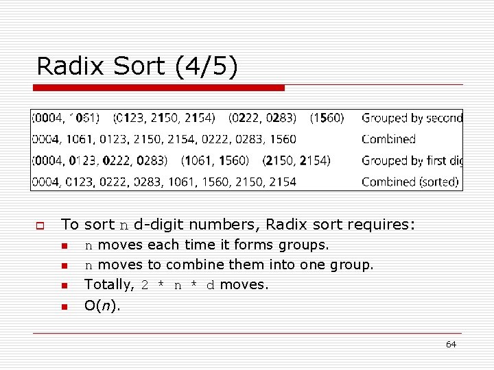
Radix Sort (3/5) n n Combine the groups into one. Next, for new groups as before, but this time use the next-to-last digits. 63

Radix Sort (4/5) o To sort n d-digit numbers, Radix sort requires: n n moves each time it forms groups. n moves to combine them into one group. Totally, 2 * n * d moves. n O(n). n n 64

Radix Sort (5/5) o Despite its efficiency, radix sort has some difficulties that make it inappropriate as a general-purpose sorting algorithm. n n n To sort integers, you need to accommodate 10 groups (0, 1, …, 9). Each group must be able to hold n strings. For large n, this requirement demands substantial memory!! 65

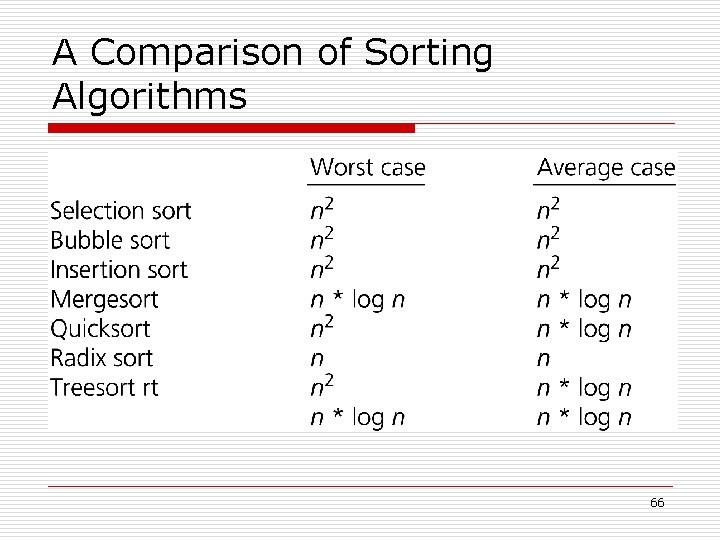
A Comparison of Sorting Algorithms 66

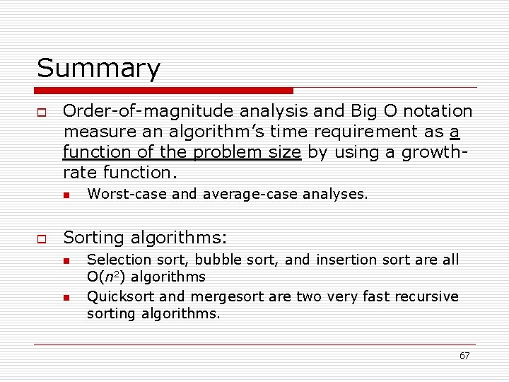
Summary o Order-of-magnitude analysis and Big O notation measure an algorithm’s time requirement as a function of the problem size by using a growthrate function. n o Worst-case and average-case analyses. Sorting algorithms: n n Selection sort, bubble sort, and insertion sort are all O(n 2) algorithms Quicksort and mergesort are two very fast recursive sorting algorithms. 67

Homework 8 o Exercises 16 and 18. (due date: 12/17) 68