COSC 3100 Fundamentals of Analysis of Algorithm Efficiency

COSC 3100 Fundamentals of Analysis of Algorithm Efficiency Instructor: Tanvir

Outline (Ch 2) • Input size, Orders of growth, Worst-case, Best-case, Average-case (Sec 2. 1) • Asymptotic notations and Basic efficiency classes (Sec 2. 2) • Analysis of Nonrecursive Algorithms (Sec 2. 3) • Analysis of Recursive Algoithms (Sec 2. 4) • Example: Computing n-th Fibonacci Number (Sec 2. 5) • Empirical Analysis, Algorithm Visualization (Sec 2. 6, 2. 7)

Analysis of Algoithms • An investigation of an algorithm’s efficiency with respect to two resources: – Running time (time efficiency or time complexity) – Memory space (space efficiency or space complexity)

Analysis Framework • Measuring an input’s size • Measuring Running Time • Orders of Growth (of algorithm’s efficiency function) • Worst-case, Best-case, and Averagecase efficiency

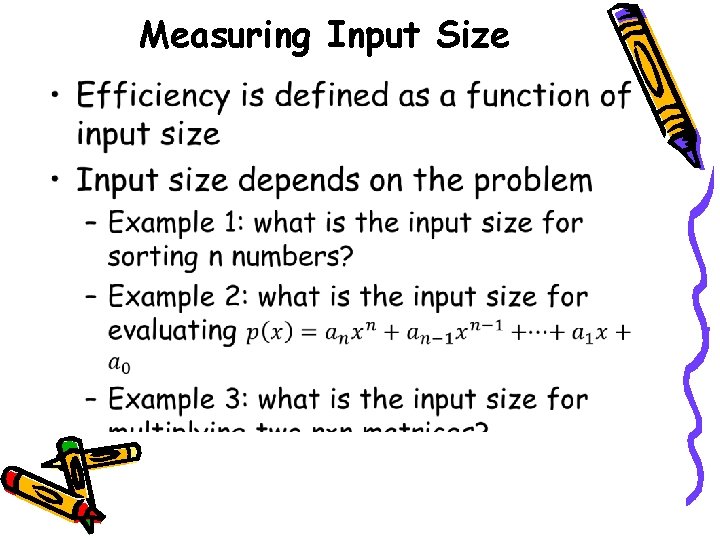
Measuring Input Size •

Units of measuring running time • Measure running time in milliseconds, etc. – Depends on which computer • Count the number of times each operation is executed – Difficult and unnecessary • Count the number of times an algorithm’s “basic operation” is executed

Measure running time in terms of # of basic operations • Basic operation: the operation that contributes the most to the total running time of an algorithm • Usually the most time consuming operation in the algorithm’s innermost loop

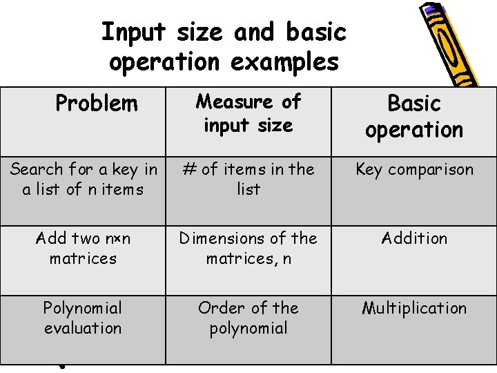
Input size and basic operation examples Problem Measure of input size Basic operation Search for a key in a list of n items # of items in the list Key comparison Add two n×n matrices Dimensions of the matrices, n Addition Polynomial evaluation Order of the polynomial Multiplication

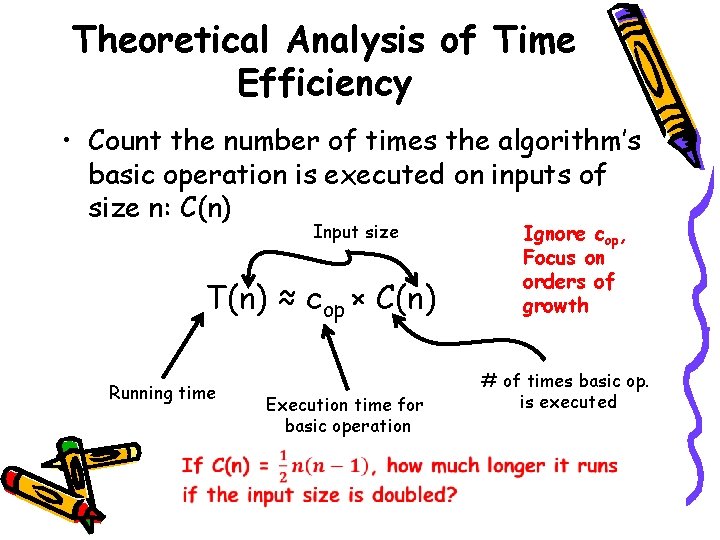
Theoretical Analysis of Time Efficiency • Count the number of times the algorithm’s basic operation is executed on inputs of size n: C(n) Input size T(n) ≈ cop × C(n) Running time Execution time for basic operation Ignore cop, Focus on orders of growth # of times basic op. is executed

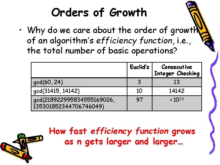
Orders of Growth • Why do we care about the order of growth of an algorithm’s efficiency function, i. e. , the total number of basic operations? Euclid’s Consecutive Integer Checking gcd(60, 24) 3 13 gcd(31415, 14142) 10 14142 gcd(218922995834555169026, 135301852344706746049) 97 > 1020 How fast efficiency function grows as n gets larger and larger…

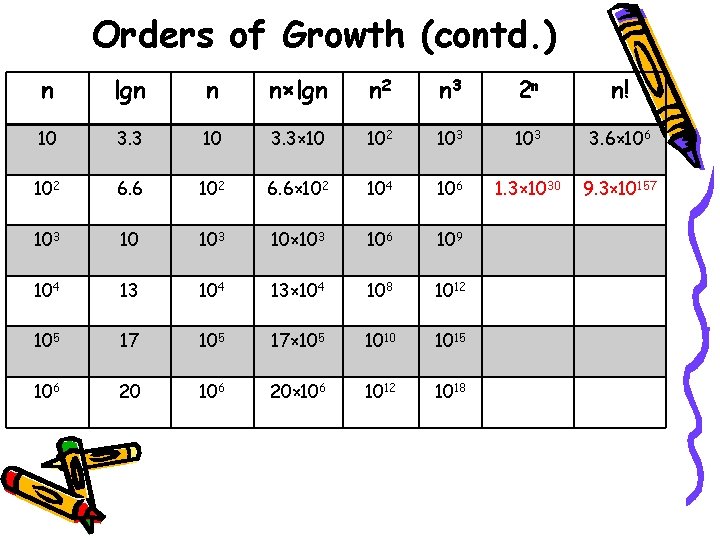
Orders of Growth (contd. ) n lgn n n×lgn n 2 n 3 2 n n! 10 3. 3× 10 102 103 3. 6× 106 102 6. 6× 102 104 106 1. 3× 1030 9. 3× 10157 103 10× 103 106 109 104 13× 104 108 1012 105 17× 105 1010 1015 106 20× 106 1012 1018

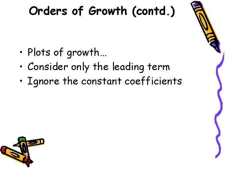
Orders of Growth (contd. ) • Plots of growth… • Consider only the leading term • Ignore the constant coefficients

Worst, Best, Average Cases • Efficiency depends on input size n • For some algorithms, efficiency depends on the type of input • Example: Sequential Search – Given a list of n elements and a search key k, find if k is in the list – Scan list, compare elements with k until either found a match (success), or list is exhausted (failure)

Sequential Search Algorithm ALGORITHM Sequential. Search(A[0. . n-1], k) //Input: A[0. . n-1] and k //Output: Index of first match or -1 if no match is //found i <- 0 while i < n and A[i] ≠ k do i <- i+1 if i < n return i //A[i] = k else return -1

Different cases • Worst case efficiency – Efficiency (# of times the basic op. will be executed) for the worst case input of size n – Runs longest among all possible inputs of size n • Best case efficiency – Runs fastest among all possible inputs of size n • Average case efficiency – Efficiency for a typical/random input of size n – NOT the average of worst and best cases – How do we find average case efficiency?

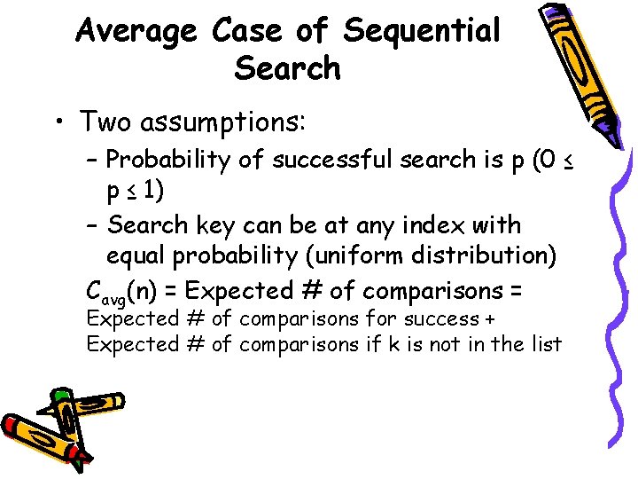
Average Case of Sequential Search • Two assumptions: – Probability of successful search is p (0 ≤ p ≤ 1) – Search key can be at any index with equal probability (uniform distribution) Cavg(n) = Expected # of comparisons for success + Expected # of comparisons if k is not in the list

Summary of Analysis Framework • Time and space efficiencies are functions of input size • Time efficiency is # of times basic operation is executed • Space efficiency is # of extra memory units consumed • Efficiencies of some algorithms depend on type of input: requiring worst, best, average case analysis • Focus is on order of growth of running time (or extra memory units) as input size goes to infinity

Asymptotic Growth Rate • 3 notations used to compare orders of growth of an algorithm’s basic operation count – O(g(n)): Set of functions that grow no faster than g(n) – Ω(g(n)): Set of functions that grow at least as fast as g(n) – Θ(g(n)): Set of functions that grow at the same rate as g(n)

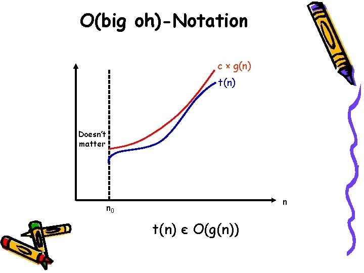
O(big oh)-Notation c × g(n) t(n) Doesn’t matter n n 0 t(n) є O(g(n))

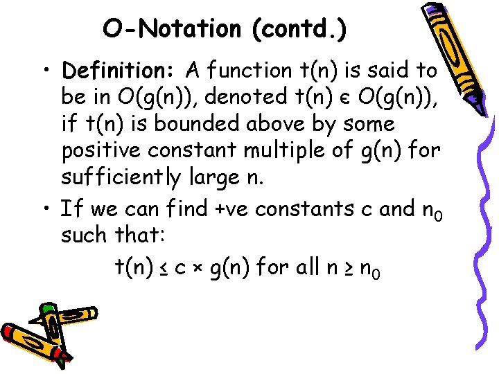
O-Notation (contd. ) • Definition: A function t(n) is said to be in O(g(n)), denoted t(n) є O(g(n)), if t(n) is bounded above by some positive constant multiple of g(n) for sufficiently large n. • If we can find +ve constants c and n 0 such that: t(n) ≤ c × g(n) for all n ≥ n 0

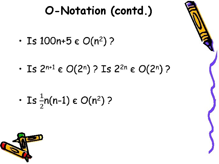
O-Notation (contd. ) •

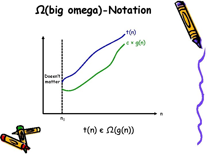
Ω(big omega)-Notation t(n) c × g(n) Doesn’t matter n n 0 t(n) є Ω(g(n))

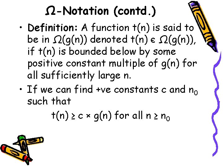
Ω-Notation (contd. ) • Definition: A function t(n) is said to be in Ω(g(n)) denoted t(n) є Ω(g(n)), if t(n) is bounded below by some positive constant multiple of g(n) for all sufficiently large n. • If we can find +ve constants c and n 0 such that t(n) ≥ c × g(n) for all n ≥ n 0

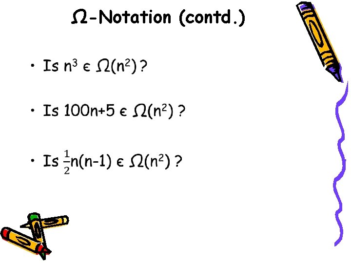
Ω-Notation (contd. ) •

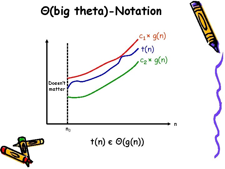
Θ(big theta)-Notation c 1 × g(n) t(n) c 2 × g(n) Doesn’t matter n n 0 t(n) є Θ(g(n))

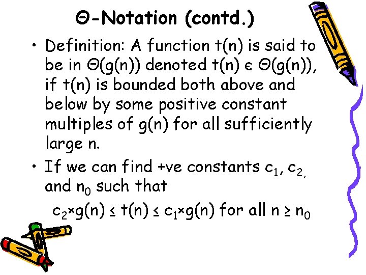
Θ-Notation (contd. ) • Definition: A function t(n) is said to be in Θ(g(n)) denoted t(n) є Θ(g(n)), if t(n) is bounded both above and below by some positive constant multiples of g(n) for all sufficiently large n. • If we can find +ve constants c 1, c 2, and n 0 such that c 2×g(n) ≤ t(n) ≤ c 1×g(n) for all n ≥ n 0

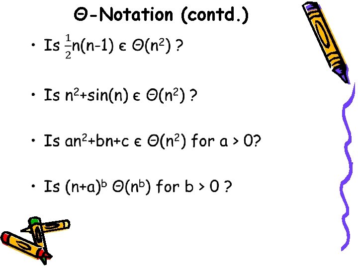
Θ-Notation (contd. ) •

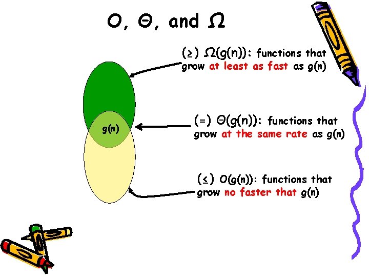
O, Θ, and Ω (≥) Ω(g(n)): functions that grow at least as fast as g(n) (=) Θ(g(n)): functions that grow at the same rate as g(n) (≤) O(g(n)): functions that grow no faster that g(n)

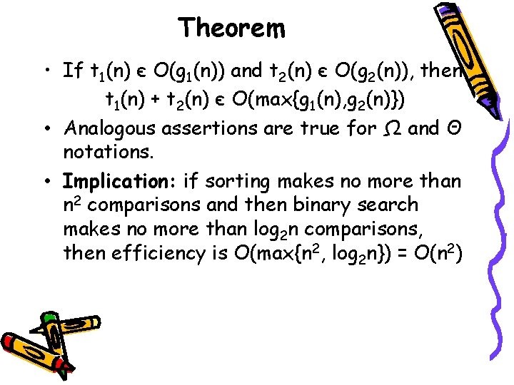
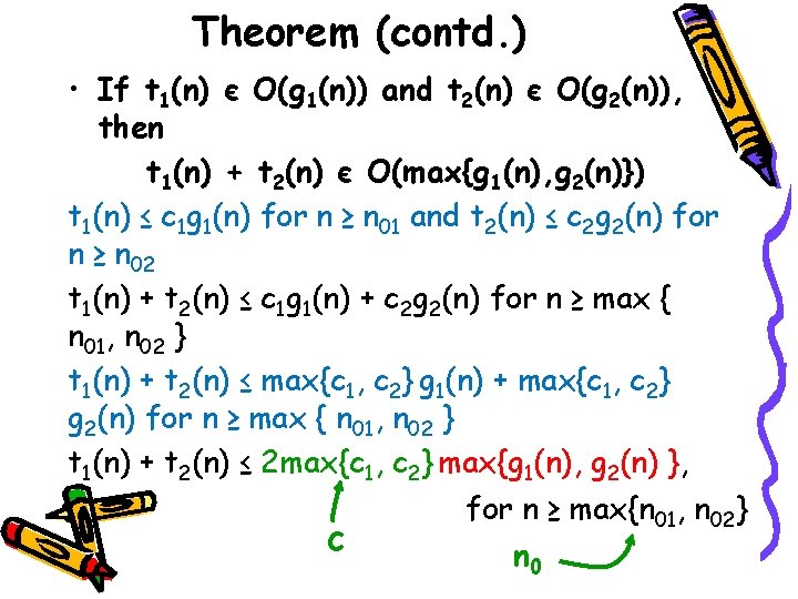
Theorem • If t 1(n) є O(g 1(n)) and t 2(n) є O(g 2(n)), then t 1(n) + t 2(n) є O(max{g 1(n), g 2(n)}) • Analogous assertions are true for Ω and Θ notations. • Implication: if sorting makes no more than n 2 comparisons and then binary search makes no more than log 2 n comparisons, then efficiency is O(max{n 2, log 2 n}) = O(n 2)

Theorem (contd. ) • If t 1(n) є O(g 1(n)) and t 2(n) є O(g 2(n)), then t 1(n) + t 2(n) є O(max{g 1(n), g 2(n)}) t 1(n) ≤ c 1 g 1(n) for n ≥ n 01 and t 2(n) ≤ c 2 g 2(n) for n ≥ n 02 t 1(n) + t 2(n) ≤ c 1 g 1(n) + c 2 g 2(n) for n ≥ max { n 01, n 02 } t 1(n) + t 2(n) ≤ max{c 1, c 2} g 1(n) + max{c 1, c 2} g 2(n) for n ≥ max { n 01, n 02 } t 1(n) + t 2(n) ≤ 2 max{c 1, c 2} max{g 1(n), g 2(n) }, for n ≥ max{n 01, n 02} c n 0

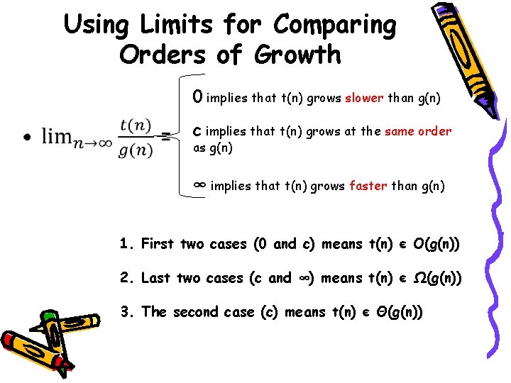
Using Limits for Comparing Orders of Growth • 0 implies that t(n) grows slower than g(n) c implies that t(n) grows at the same order as g(n) ∞ implies that t(n) grows faster than g(n) 1. First two cases (0 and c) means t(n) є O(g(n)) 2. Last two cases (c and ∞) means t(n) є Ω(g(n)) 3. The second case (c) means t(n) є Θ(g(n))

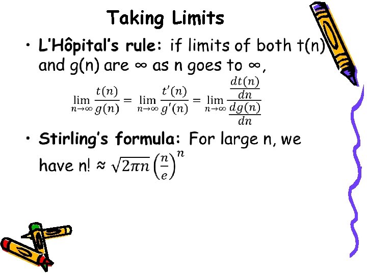
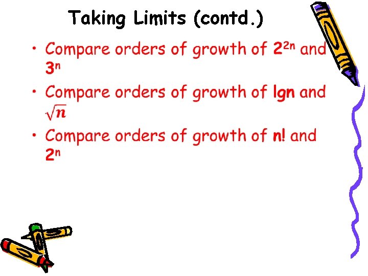
Taking Limits •

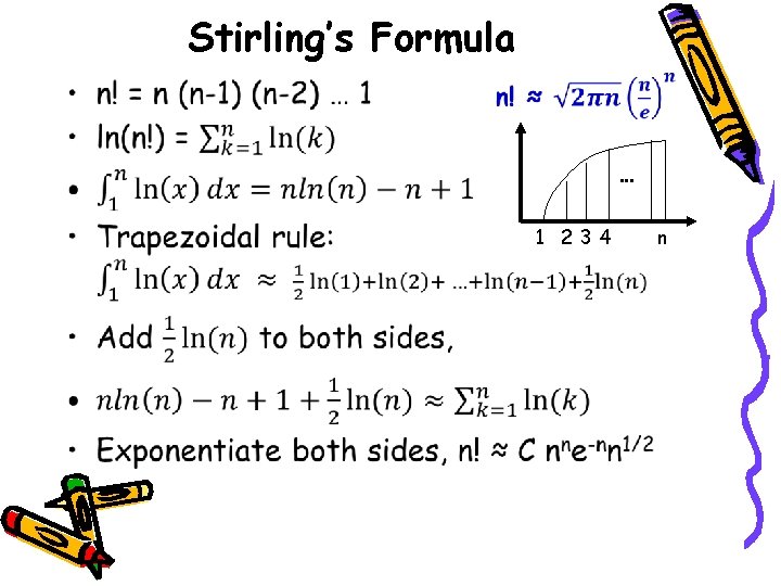
Stirling’s Formula • … 1 234 n

Taking Limits (contd. ) •

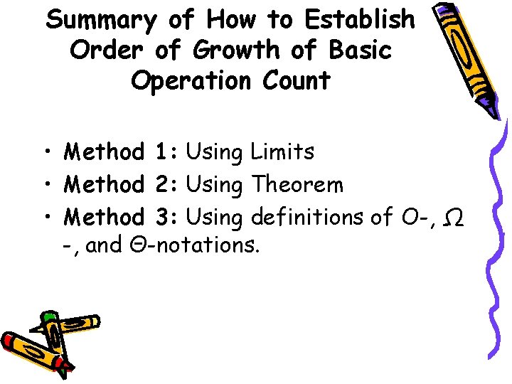
Summary of How to Establish Order of Growth of Basic Operation Count • Method 1: Using Limits • Method 2: Using Theorem • Method 3: Using definitions of O-, Ω -, and Θ-notations.

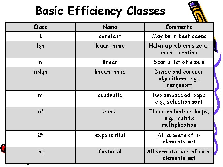
Basic Efficiency Classes Class Name Comments 1 constant May be in best cases lgn logarithmic Halving problem size at each iteration n linear Scan a list of size n n×lgn linearithmic Divide and conquer algorithms, e. g. , mergesort n 2 quadratic Two embedded loops, e. g. , selection sort n 3 cubic Three embedded loops, e. g. , matrix multiplication 2 n exponential All subsets of nelements set n! factorial All permutations of an nelements set

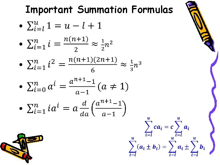
Important Summation Formulas •

Analysis of Nonrecursive Algorithms ALGORITHM Max. Element(A[0. . n-1]) //Determines largest element maxval <- A[0] Input size: n for i <- 1 to n-1 do Basic operation: > or <if A[i] > maxval <- A[i] return maxval

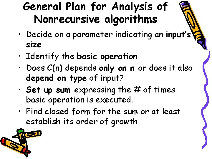
General Plan for Analysis of Nonrecursive algorithms • Decide on a parameter indicating an input’s size • Identify the basic operation • Does C(n) depends only on n or does it also depend on type of input? • Set up sum expressing the # of times basic operation is executed. • Find closed form for the sum or at least establish its order of growth

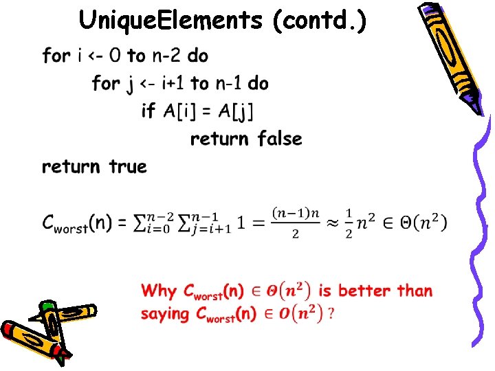
Analysis of Nonrecursive (contd. ) ALGORITHM Unique. Elements(A[0. . n-1]) //Determines whether all elements are //distinct for i <- 0 to n-2 do for j <- i+1 to n-1 do if A[i] = A[j] return false return true Input size: n Basic operation: A[i] = A[j] Does C(n) depend on type of input?

Unique. Elements (contd. ) •

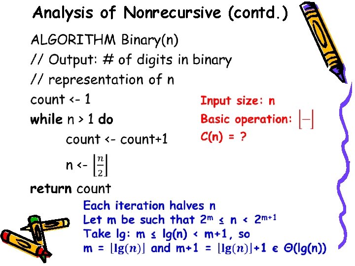
Analysis of Nonrecursive (contd. ) ALGORITHM Matrix. Multiplication(A[0. . n-1, 0. . n-1], B[0. . n-1, 0. . n-1]) //Output: C = AB T(n) ≈ cm. M(n)+ca. A(n) for i <- 0 to n-1 do 3+c n 3 = c n m a for j <- 0 to n-1 do 3 = (c +c )n m a C[i, j] = 0. 0 for k <- 0 to n-1 do C[i, j] = C[i, j] + A[i, k]×B[k, j] return C

Analysis of Nonrecursive (contd. ) •

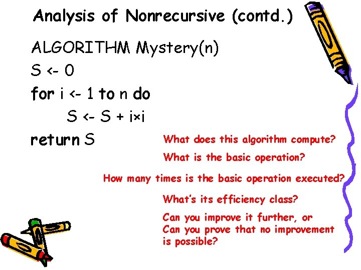
Analysis of Nonrecursive (contd. ) ALGORITHM Mystery(n) S <- 0 for i <- 1 to n do S <- S + i×i What does this algorithm compute? return S What is the basic operation? How many times is the basic operation executed? What’s its efficiency class? Can you improve it further, or Can you prove that no improvement is possible?

Analysis of Nonrecursive (contd. ) ALGORITHM Secret(A[0. . n-1]) r <- A[0] What does this algorithm compute? s <- A[0] What is the basic operation? for i <- 1 to n-1 do if A[i] < r How many times is the basic operation executed? r <- A[i] if A[i] > s What’s its efficiency class? s <- A[i] return s-r Can you improve it further, Or Could you prove that no improvement is possible?

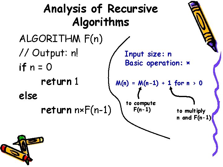
Analysis of Recursive Algorithms ALGORITHM F(n) // Output: n! if n = 0 return 1 else return n×F(n-1) Input size: n Basic operation: × M(n) = M(n-1) + 1 for n > 0 to compute F(n-1) to multiply n and F(n-1)

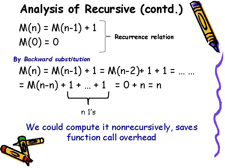
Analysis of Recursive (contd. ) M(n) = M(n-1) + 1 M(0) = 0 Recurrence relation By Backward substitution M(n) = M(n-1) + 1 = M(n-2)+ 1 = … … = M(n-n) + 1 + … + 1 = 0 + n = n n 1’s We could compute it nonrecursively, saves function call overhead

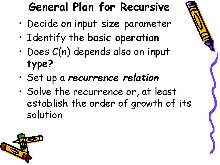
General Plan for Recursive • Decide on input size parameter • Identify the basic operation • Does C(n) depends also on input type? • Set up a recurrence relation • Solve the recurrence or, at least establish the order of growth of its solution

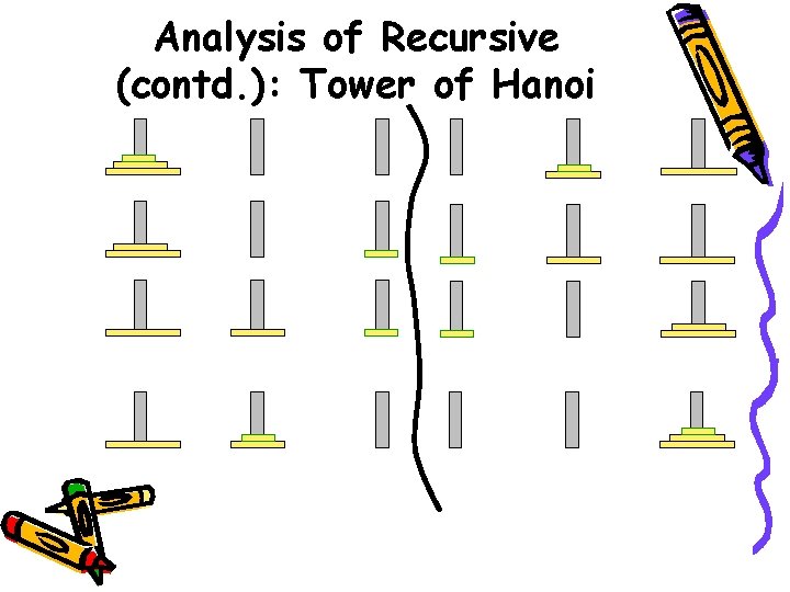
Analysis of Recursive (contd. ): Tower of Hanoi

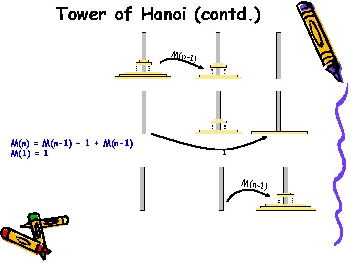
Tower of Hanoi (contd. ) M(n-1) M(n) = M(n-1) + 1 + M(n-1) M(1) = 1 1 M(n-1)

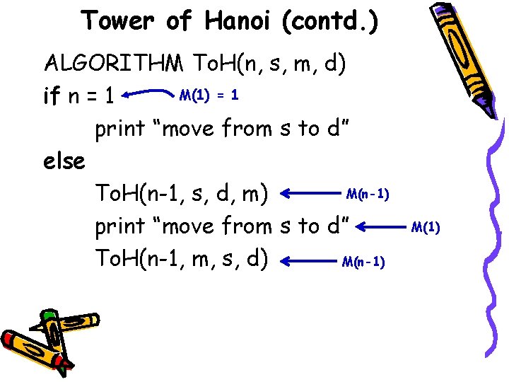
Tower of Hanoi (contd. ) ALGORITHM To. H(n, s, m, d) M(1) = 1 if n = 1 print “move from s to d” else M(n-1) To. H(n-1, s, d, m) print “move from s to d” M(n-1) To. H(n-1, m, s, d) M(1)

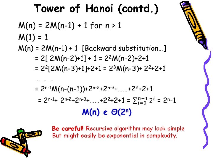
Tower of Hanoi (contd. ) • Be careful! Recursive algorithm may look simple But might easily be exponential in complexity.

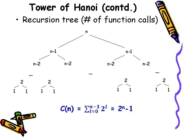
Tower of Hanoi (contd. ) • Recursion tree (# of function calls) n n-1 n-2 n-2 … … 2 1 n-2 2 2 1 1 … 1 1 2 1 1 1

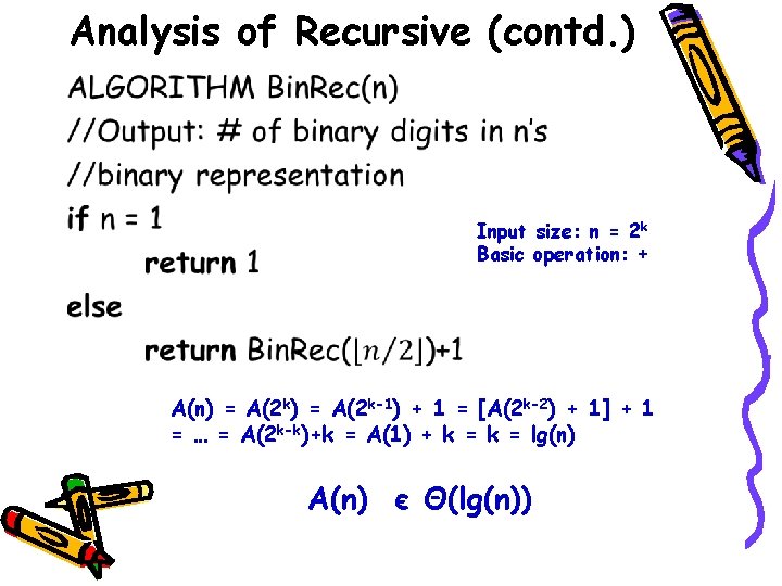
Analysis of Recursive (contd. ) • Input size: n = 2 k Basic operation: + A(n) = A(2 k-1) + 1 = [A(2 k-2) + 1] + 1 = … = A(2 k-k)+k = A(1) + k = lg(n) A(n) є Θ(lg(n))

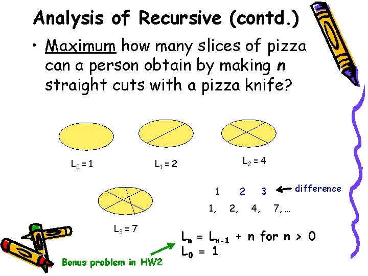
Analysis of Recursive (contd. ) • Maximum how many slices of pizza can a person obtain by making n straight cuts with a pizza knife? L 0 = 1 L 2 = 4 L 1 = 2 1 1, L 3 = 7 Bonus problem in HW 2 2 2, difference 3 4, 7, … Ln = Ln-1 + n for n > 0 L 0 = 1

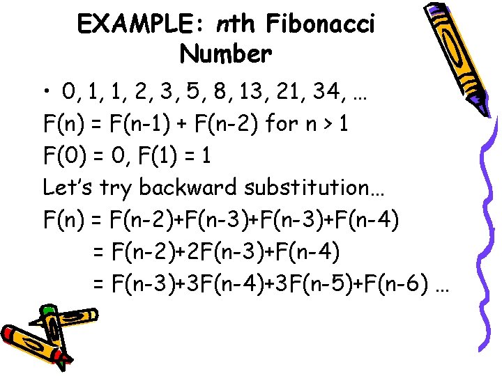
EXAMPLE: nth Fibonacci Number • 0, 1, 1, 2, 3, 5, 8, 13, 21, 34, … F(n) = F(n-1) + F(n-2) for n > 1 F(0) = 0, F(1) = 1 Let’s try backward substitution… F(n) = F(n-2)+F(n-3)+F(n-4) = F(n-2)+2 F(n-3)+F(n-4) = F(n-3)+3 F(n-4)+3 F(n-5)+F(n-6) …

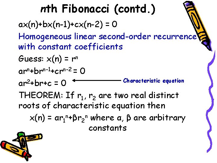
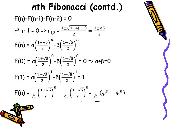
nth Fibonacci (contd. ) ax(n)+bx(n-1)+cx(n-2) = 0 Homogeneous linear second-order recurrence with constant coefficients Guess: x(n) = rn arn+brn-1+crn-2 = 0 Characteristic equation ar 2+br+c = 0 THEOREM: If r 1, r 2 are two real distinct roots of characteristic equation then x(n) = αr 1 n+βr 2 n where α, β are arbitrary constants

nth Fibonacci (contd. ) •

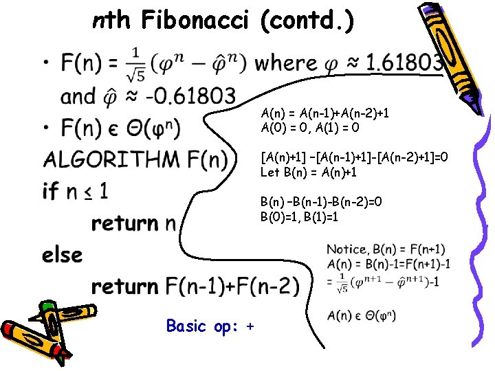
nth Fibonacci (contd. ) • A(n) = A(n-1)+A(n-2)+1 A(0) = 0, A(1) = 0 [A(n)+1] –[A(n-1)+1]-[A(n-2)+1]=0 Let B(n) = A(n)+1 B(n) –B(n-1)-B(n-2)=0 B(0)=1, B(1)=1 Basic op: +

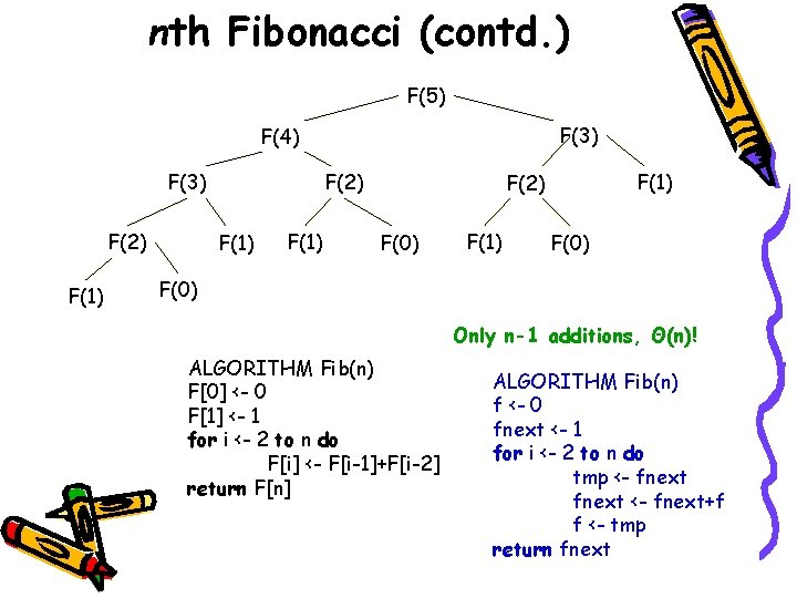
nth Fibonacci (contd. ) F(5) F(3) F(4) F(3) F(2) F(1) F(2) F(0) F(1) F(0) Only n-1 additions, Θ(n)! ALGORITHM Fib(n) F[0] <- 0 F[1] <- 1 for i <- 2 to n do F[i] <- F[i-1]+F[i-2] return F[n] ALGORITHM Fib(n) f <- 0 fnext <- 1 for i <- 2 to n do tmp <- fnext+f f <- tmp return fnext

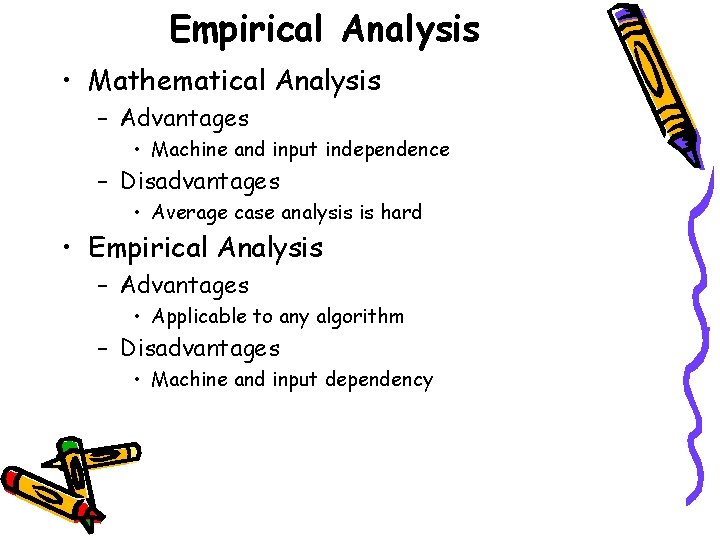
Empirical Analysis • Mathematical Analysis – Advantages • Machine and input independence – Disadvantages • Average case analysis is hard • Empirical Analysis – Advantages • Applicable to any algorithm – Disadvantages • Machine and input dependency

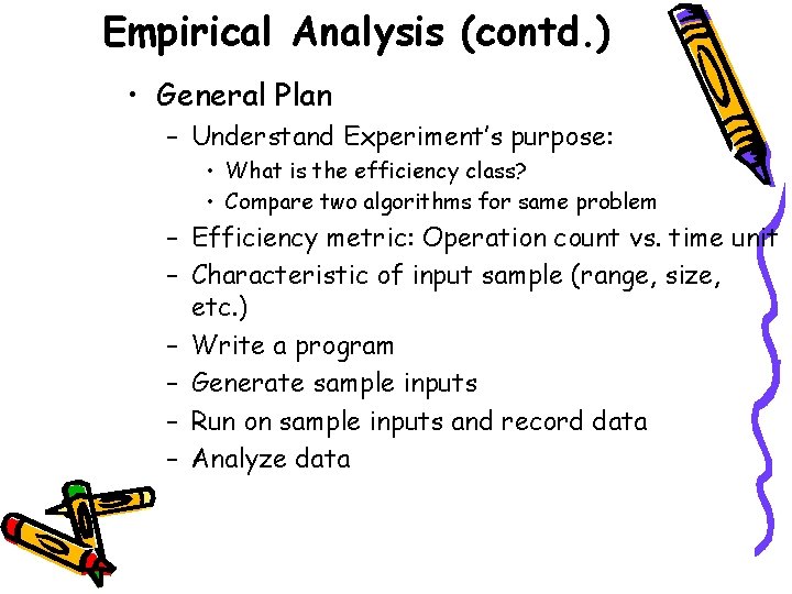
Empirical Analysis (contd. ) • General Plan – Understand Experiment’s purpose: • What is the efficiency class? • Compare two algorithms for same problem – Efficiency metric: Operation count vs. time unit – Characteristic of input sample (range, size, etc. ) – Write a program – Generate sample inputs – Run on sample inputs and record data – Analyze data

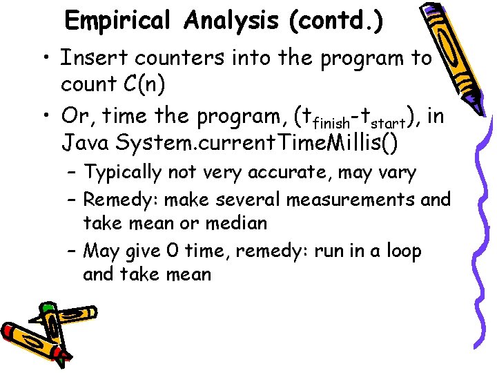
Empirical Analysis (contd. ) • Insert counters into the program to count C(n) • Or, time the program, (tfinish-tstart), in Java System. current. Time. Millis() – Typically not very accurate, may vary – Remedy: make several measurements and take mean or median – May give 0 time, remedy: run in a loop and take mean

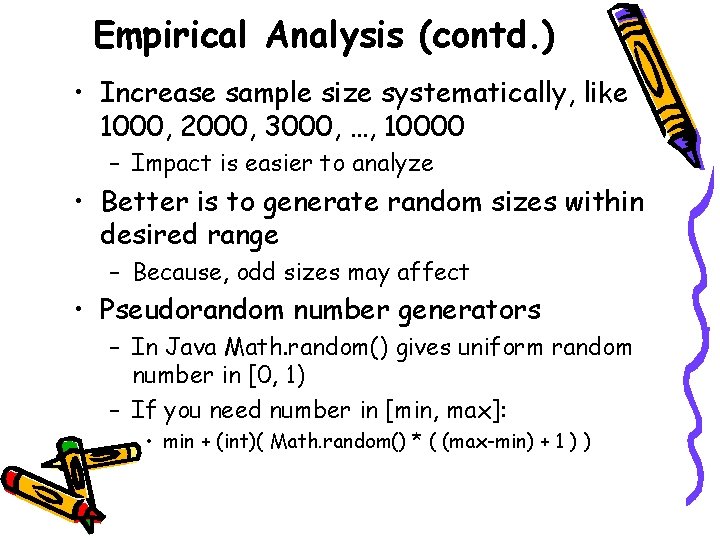
Empirical Analysis (contd. ) • Increase sample size systematically, like 1000, 2000, 3000, …, 10000 – Impact is easier to analyze • Better is to generate random sizes within desired range – Because, odd sizes may affect • Pseudorandom number generators – In Java Math. random() gives uniform random number in [0, 1) – If you need number in [min, max]: • min + (int)( Math. random() * ( (max-min) + 1 ) )

Empirical Analysis (contd. ) • Pseudorandom in [min, max] – Math. random() * (max-min) gives [0, max-min) – min + Math. random() * (max-min) gives [min, max) – (int)[Math. random() * (max-min+1)] gives [0, max-min] – min+ (int)[Math. random() * (max-min+1)] gives [min, max] • To get [5, 10] – (int)Math. random()*(10 -5+1) gives [0, 10 -5] or [0, 5] – 5+ (int)Math. random()*(10 -5+1) gives [5, 10]

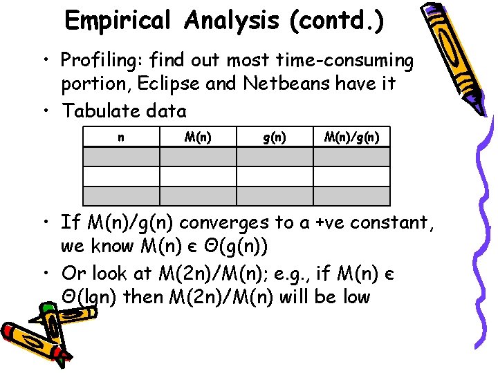
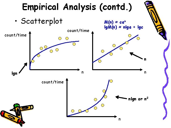
Empirical Analysis (contd. ) • Profiling: find out most time-consuming portion, Eclipse and Netbeans have it • Tabulate data n M(n) g(n) M(n)/g(n) • If M(n)/g(n) converges to a +ve constant, we know M(n) є Θ(g(n)) • Or look at M(2 n)/M(n); e. g. , if M(n) є Θ(lgn) then M(2 n)/M(n) will be low

Empirical Analysis (contd. ) • Scatterplot count/time M(n) ≈ can lg. M(n) ≈ nlga + lgc n n lgn n count/time nlgn or n 2 n

Algorithm Visualization (contd. ) • Sequence of still pictures or animation • Sorting Out Sorting on You. Tube – Nice animation of 9 sorting algorithms

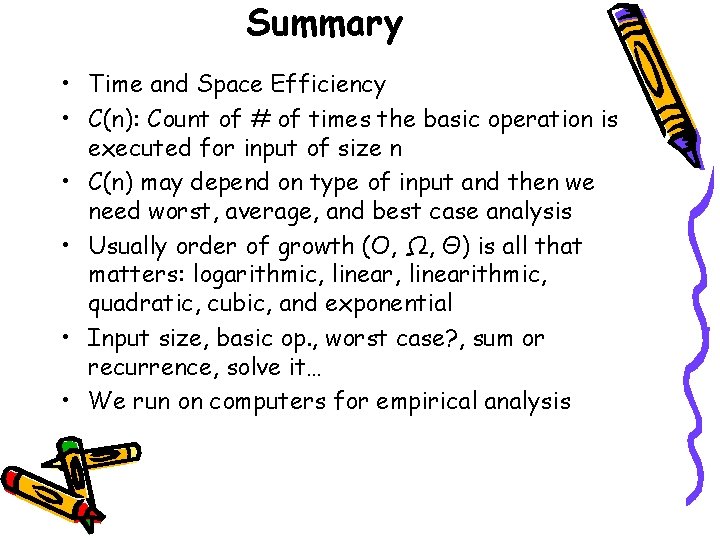
Summary • Time and Space Efficiency • C(n): Count of # of times the basic operation is executed for input of size n • C(n) may depend on type of input and then we need worst, average, and best case analysis • Usually order of growth (O, Ω, Θ) is all that matters: logarithmic, linearithmic, quadratic, cubic, and exponential • Input size, basic op. , worst case? , sum or recurrence, solve it… • We run on computers for empirical analysis

Homework 2 • DUE ON FEBRUARY 07 (TUESDAY) IN CLASS