Fundamentals of the Analysis of Algorithm Efficiency 2

Fundamentals of the Analysis of Algorithm Efficiency 2. 1 2. 2 2. 3 2. 4 Algorithm analysis framework Asymptotic notations Analysis of non-recursive algorithms Analysis of recursive algorithms

Analysis of Algorithms Analysis of algorithms means to investigate an algorithm’s efficiency with respect to resources: running time and memory space. Time efficiency: how fast an algorithm runs. Space efficiency: the space an algorithm requires. Typically, algorithms run longer as the size of its input increases We are interested in how efficiency scales wrt input size

2. 1 Analysis Framework Measuring an input’s size Measuring running time Orders of growth (of the algorithm’s efficiency function) Worst-case, best-case and average-case efficiency

Measuring Input Sizes Almost all algorithms run longer on larger inputs. Therefore, it is logical to investigate an algorithm’s efficiency as a function of some parameter n indicating the algorithm’s input size. Input size depends on the problem. § Example 1: what is the input size of the problem of sorting n numbers? § Example 2: what is the input size of adding two n by n matrices?

Units for Measuring Running Time The next issues concerns units for measuring an algorithm’s running time. Should we measure the running time using standard unit of time measurements, such as seconds, minutes? However: § Depends on the speed of the computer. § Depends on the quality of a program implementing the algorithm One possible approach is to count the number of times each of the algorithm’s operations is executed. § Difficult and usually unnecessary Count the number of times an algorithm’s basic operation is executed. § Basic operation: the operation that contributes the most to the total running time. § For example, the basic operation is usually the most time-consuming operation in the algorithm’s innermost loop.

Order of growth Most important: Order of growth within a constant multiple as n→∞ Example: § How much faster will algorithm run on computer that is twice as fast? § How much longer does it take to solve problem of double input size?

Input size and basic operation examples Problem Input size measure Basic operation Searching for key in a list of n items Number of list’s items, i. e. n Key comparison Multiplication of two matrices Matrix dimensions or total number of elements Multiplication of two numbers Checking primality of a given integer n n’size = number of digits Division (in binary representation) Typical graph problem #vertices and/or edges Visiting a vertex or traversing an edge

Theoretical Analysis of Time Efficiency Time efficiency is analyzed by determining the number of repetitions of the basic operation as a function of input size. Assuming C(n) = (1/2)n(n-1) ≈ (½) n 2 how much longer will the algorithm run if we double the input size? The answer is about four times longer. (page 45) input size T(n) ≈ cop. C (n) running time execution time for the basic operation Number of times the basic operation is executed The efficiency analysis framework ignores the multiplicative constants of C(n) and focuses on the orders of growth of the C(n).

Orders of Growth Exponential-growth functions Orders of growth: consider only the leading term of a formula ignore the constant coefficient.

Worst-Case, Best-Case, and Average. Case Efficiency Algorithm efficiency depends on the input size n For some algorithms efficiency depends on type of input. § Example: Sequential Search – Problem: Given a list of n elements and a search key K, find an element equal to K, if any. – Algorithm: Scan the list and compare its successive elements with K until either a matching element is found (successful search) or the list is exhausted (unsuccessful search) Given a sequential search problem of an input size of n, what kind of input would make the running time the longest? How many key comparisons?

Sequential Search Algorithm ALGORITHM Sequential. Search(A[0. . n-1], K) //Searches for a given value in a given array by sequential search //Input: An array A[0. . n-1] and a search key K //Output: Returns the index of the first element of A that matches K or – 1 if there are no matching elements i 0 while i < n and A[i] ≠ K do i i+1 if i < n //A[I] = K return i else return -1 Clearly, the running time of this algorithm can be quite different for the same list size n. for that we need to distinguish between the worst-case, best case and average-case efficiencies.

Worst-Case, Best-Case, and Average-Case Efficiency Worst case Efficiency § Efficiency (# of times the basic operation will be executed) for the worst case input of size n. § The algorithm runs the longest among all possible inputs of size n. Best case § Efficiency (# of times the basic operation will be executed) for the best case input of size n. § The algorithm runs the fastest among all possible inputs of size n. Average case: § Efficiency (#of times the basic operation will be executed) for a typical/random input of size n. § NOT the average of worst and best case § How to find the average case efficiency?

Summary of the Analysis Framework Both time and space efficiencies are measured as functions of input size. Time efficiency is measured by counting the number of basic operations executed in the algorithm. The space efficiency is measured by the number of extra memory units consumed. The framework’s primary interest lies in the order of growth of the algorithm’s running time (space) as its input size goes infinity. The efficiencies of some algorithms may differ significantly for inputs of the same size. For these algorithms, we need to distinguish between the worst-case, best-case and average case efficiencies.

2. 2 Asymptotic Notations To compare and rank order of growth of algorithm’s basic operation count, computer scientist use three notations: O (big oh), Ω (big omega) and Θ (big theta). Informally, O(g(n)) is the set of all functions with a smaller or same order of growth as g(n). Ω(g(n)) stands for the set of all functions with a larger or same order of growth as g(n). Θ(g(n)) is the set of all functions that have the same order of growth as g(n).

O-notation

O-notation Suppose t(n) and g(n) can be any nonnegative functions defined on the set of natural numbers. t(n) will be an algorithm’s running time and g(n) will be some simple function to compare the count with. Formal definition § A function t(n) is said to be in O(g(n)), denoted t(n) O(g(n)), if t(n) is bounded above by some constant multiple of g(n) for all large n, i. e. , if there exist some positive constant c and some nonnegative integer n 0 such that t(n) cg(n) for all n n 0 The definition is illustrated in figure above.

-notation

-notation Formal definition § A function t(n) is said to be in (g(n)), denoted t(n) (g(n)), if t(n) is bounded below by some constant multiple of g(n) for all large n, i. e. , if there exist some positive constant c and some nonnegative integer n 0 such that t(n) cg(n) for all n n 0 Here is an example for the formal proof that n 3 Ω(n 2) n 3 ≥ (n 2) for all n ≥ 0 i. e. , we can select c=1 and n 0 =0.

-notation

-notation Formal definition § A function t(n) is said to be in (g(n)), denoted t(n) (g(n)), if t(n) is bounded both above and below by some positive constant multiples of g(n) for all large n, i. e. , if there exist some positive constant c 1 and c 2 and some nonnegative integer n 0 such that c 2 g(n) t(n) c 1 g(n) for all n n 0 Exercises: prove the following using the above definition § 10 n 2 (n 2) § 10 n 2 + 2 n (n 2) § (1/2)n(n-1) (n 2)

>= (g(n)), functions that grow at least as fast as g(n) = g(n) (g(n)), functions that grow at the same rate as g(n) <= O(g(n)), functions that grow no faster than g(n)

Some Properties of Asymptotic Order of Growth 1. f(n) O(f(n)) 2. f(n) O(g(n)) iff g(n) (f(n)) 3. If f (n) O(g (n)) and g(n) O(h(n)) , then f(n) O(h(n)) Note similarity with a ≤ b 4. If f 1(n) O(g 1(n)) and f 2(n) O(g 2(n)) , then f 1(n) + f 2(n) O(max{g 1(n), g 2(n)}) The analogous assertions are true for the -notation and notation.

Some Properties of Asymptotic Order of Growth If f 1(n) O(g 1(n)) and f 2(n) O(g 2(n)) , then f 1(n) + f 2(n) O(max{g 1(n), g 2(n)}) Implication: The algorithm’s overall efficiency will be determined by the part with a larger order of growth. § For example, – 5 n 2 + 3 nlogn O(n 2)

Using Limits for Comparing Orders of Growth 0 order of growth of t(n) limn→∞ t(n)/g(n) = < order of growth of g(n) c order of growth of t(n) = order of growth of g(n) ∞ order of growth of t(n) > order of growth of g(n) See the Example on page 57 Anany Levitin

L’Hôpital’s rule If limn→∞ f(n) = limn→∞ g(n) = ∞ and the derivatives f ´, g ´ exist, Then f(n ) f ´(n) lim = g ( n ) n→∞ g ´(n) Stirling’s formula: n! (2 n)1/2 (n/e)n

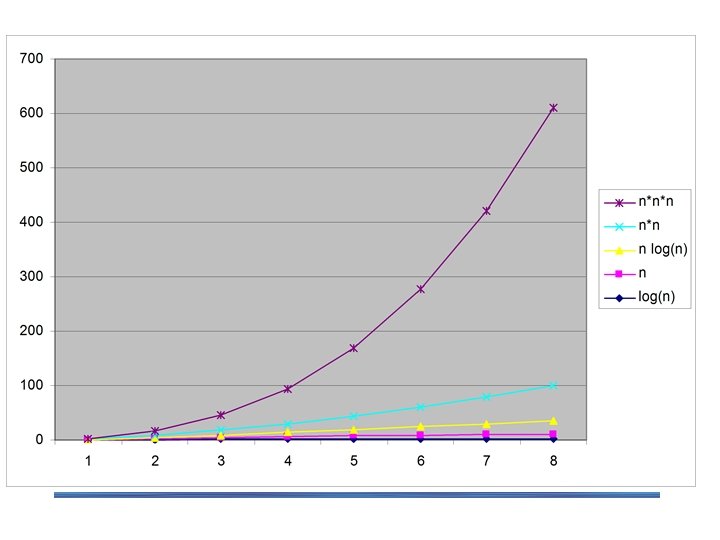
Basic Efficiency classes fast slow 1 constant log n logarithmic n linear n log n n 2 quadratic n 3 cubic 2 n exponential n! factorial The time efficiencies of a large number of algorithms fall into only a few classes. High time efficiency low time efficiency

2. 3 Time Efficiency of Nonrecursive Algorithms Steps in mathematical analysis of non-recursive algorithms: Decide on parameter n indicating input size Identify algorithm’s basic operation Check whether the number of times the basic operation is executed depends only on the input size n. If it also depends on the type of input, investigate worst, average, and best case efficiency separately. Set up summation for C(n) reflecting the number of times the algorithm’s basic operation is executed. Simplify summation using standard formulas (see Appendix A)

Example 1: Maximum Element Consider the problem of finding the value of the largest element in a list of n numbers. We assume that list is implemented as array. The following is a pseudocode of a standard algorithm for solving the problem:

Example 1: Maximum Element The obvious measure of an input’s size here is number of elements in the array, i. e. , n. the operations that are going to be executed most often are in the algorithm’s for loop. There are two operations in the loop’s body: the comparison A[i]>maxval and the assignment maxval ← A[i]. Which of the two operations should be considered as basic? Since the comparison is executed on each repetition of the loop and the assignment is not. So comparison is basic operation. The algorithm makes one comparison on each execution of the loop, therefore we get the following sum for C(n): C(n) = (i=1 to n-1)∑ 1 = n-1 Θ(n)

Example 2: Element Uniqueness Problem Consider the element uniqueness problem: check whether all the elements in a given array are distinct. The following is a pseudocode of a standard algorithm for solving the problem: In the worst-case, the algorithm needs to compare all n(n-1)/2 distinct pairs of its n elements.

Example 3: Matrix multiplication Given two n-by-n matrices A and B, find the time efficiency of the definition based algorithm for computing their product C = AB.

Example 3: Matrix multiplication We measure an input’s size by matrix order n. The algorithm’s innermost loop are two arithmetical operations-multiplication and addition. We consider multiplications the algorithm’s basic operation. The number of multiplications made for every pair of specific values of variables i and j is (k=0 to n-1) ∑ 1 And total number of multiplications M(n) is expressed by the following triple sum: M(n) = (i=0 to n-1)∑ (j=0 to n-1)∑ (k=0 to n-1)∑ 1 = (i=0 to n-1)∑ (j=0 to n-1)∑ n = (i=0 to n-1)∑ n 2 = n 3 So the running time of algorithm T(n) ≈ cm M(n) = cm n 3 Where cm is the time of one multiplication

Example 4: Counting binary digits The most frequently executed operation here is not inside the while loop but rather the comparison n > 1 that determined whether the loop’s body will be executed. It cannot be investigated the way the previous examples are. We will analyze it in the following part.

2. 4 Mathematical Analysis of Recursive Algorithms Recursive evaluation of n! Recursive solution to the Towers of Hanoi puzzle Recursive solution to the number of binary digits problem

Example 1: Recursive evaluation of n ! Iterative Definition F(n) = 1 = n * (n-1) * (n-2)… 3 * 2 * 1 Recursive definition F(n) = 1 F(n) = n * F(n-1) if n = 0 if n > 0 § Algorithm F(n) if n=0 return 1 //base case return F (n -1) * n //general case else

Example 1: Recursive evaluation of n ! We consider n itself an indicator of this algorithm’s input size. The basic operation is multiplication, whose number of executions we denote M(n). Since the function F(n) is computed according to the formula F(n) = F(n-1). n for n > 0 So, M(n) = M(n-1) + 1 for n > 0 Condition that makes the algorithms stop its recursive calls: if n = 0 return 1 When n = 0 the algorithm performs no multiplications M(0) = 0 Finally, M(n) ∈ Θ (n)

Steps in Mathematical Analysis of Recursive Algorithms Decide on parameter n indicating input size Identify algorithm’s basic operation Check whether the number of times the basic operation is executed may vary on different inputs of the same size. (If it may, the worst, average, and best cases must be investigated separately. ) Set up a recurrence relation and initial condition(s) for C(n)-the number of times the basic operation will be executed for an input of size n (alternatively count recursive calls). Solve the recurrence or estimate the order of magnitude of the solution by backward substitutions or another method (see Appendix B)

Example 2: The Tower of Hanoi Puzzle In this puzzle, we have n disks of different sizes and three pegs. Initially all the disks are on the first peg in order of size, the largest on the bottom and the smallest on top.

The Towers of Hanoi Puzzle The number of disks n is the obvious choice for the input size indicator, and so is moving one disk as the algorithm’s basic operation. Clearly the number of moves M(n) depends on n only, and we get following recurrence equation for it: M(n) = M(n – 1) + 1 + M(n - 1) for n > 1 = 2 M(n – 1) + 1 for n > 1 With initial condition, M(1) = 1 By using backward substitutions, (page 73) M(n) = 2 n – 1 Thus we have exponential algorithm, which will run for long time even for moderate values of n.

Example 3: Find the number of binary digits in the binary representation of a positive decimal integer Compute number of additions: A(n) = A( n/2 )+1 with A(1) = 0