Chapter 10 A Algorithm Efficiency Determining the Efficiency

Chapter 10 A Algorithm Efficiency

Determining the Efficiency of Algorithms • Analysis of algorithms – Provides tools for contrasting the efficiency of different methods of solution • A comparison of algorithms – Should focus of significant differences in efficiency – Should not consider reductions in computing costs due to clever coding tricks © 2004 Pearson Addison-Wesley. All rights reserved 10 A-2

Determining the Efficiency of Algorithms • Three difficulties with comparing programs instead of algorithms – How are the algorithms coded? – What computer should you use? – What data should the programs use? • Algorithm analysis should be independent of – Specific implementations – Computers – Data © 2004 Pearson Addison-Wesley. All rights reserved 10 A-3

The Execution Time of Algorithms • Counting an algorithm's operations is a way to access its efficiency – An algorithm’s execution time is related to the number of operations it requires – Examples • Traversal of a linked list • The Towers of Hanoi • Nested Loops © 2004 Pearson Addison-Wesley. All rights reserved 10 A-4

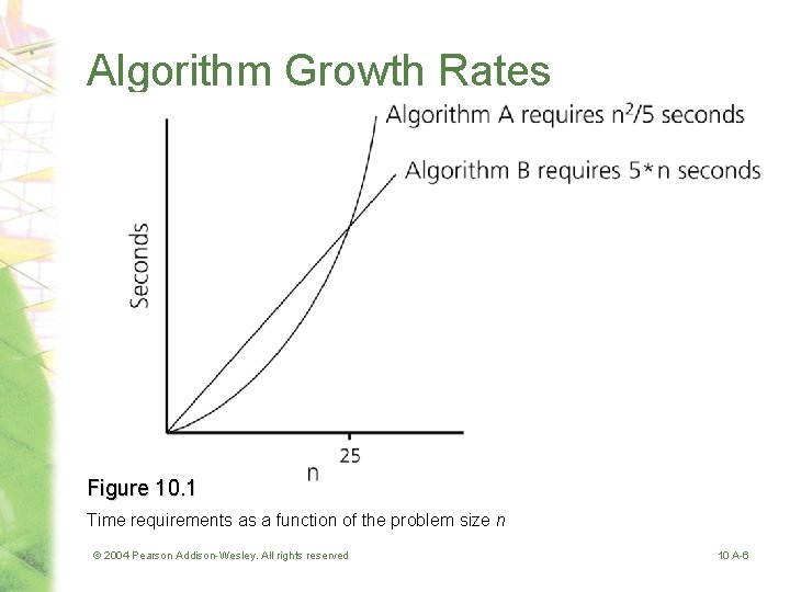
Algorithm Growth Rates • An algorithm’s time requirements can be measured as a function of the problem size • An algorithm’s growth rate – Enables the comparison of one algorithm with another – Examples Algorithm A requires time proportional to n 2 Algorithm B requires time proportional to n • Algorithm efficiency is typically a concern for large problems only © 2004 Pearson Addison-Wesley. All rights reserved 10 A-5

Algorithm Growth Rates Figure 10. 1 Time requirements as a function of the problem size n © 2004 Pearson Addison-Wesley. All rights reserved 10 A-6

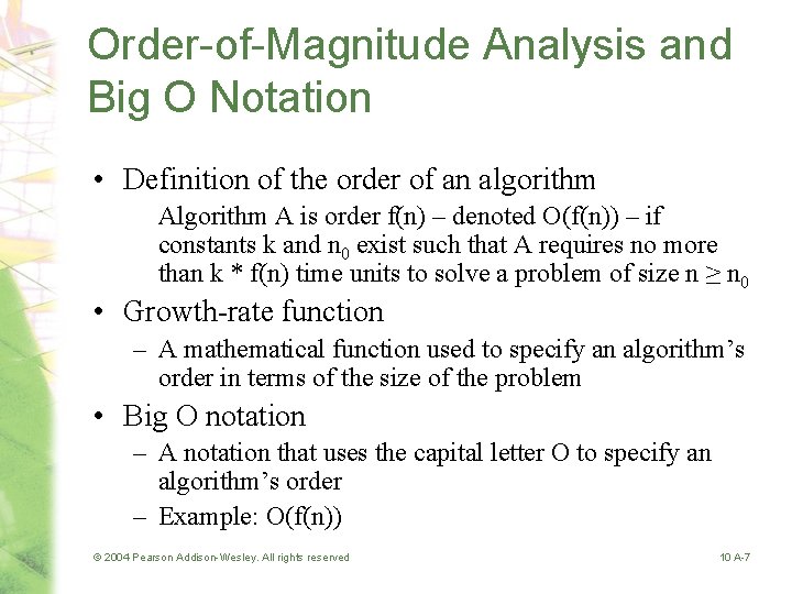
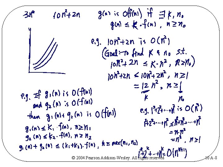
Order-of-Magnitude Analysis and Big O Notation • Definition of the order of an algorithm A is order f(n) – denoted O(f(n)) – if constants k and n 0 exist such that A requires no more than k * f(n) time units to solve a problem of size n ≥ n 0 • Growth-rate function – A mathematical function used to specify an algorithm’s order in terms of the size of the problem • Big O notation – A notation that uses the capital letter O to specify an algorithm’s order – Example: O(f(n)) © 2004 Pearson Addison-Wesley. All rights reserved 10 A-7

© 2004 Pearson Addison-Wesley. All rights reserved 10 A-8

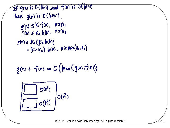
© 2004 Pearson Addison-Wesley. All rights reserved 10 A-9

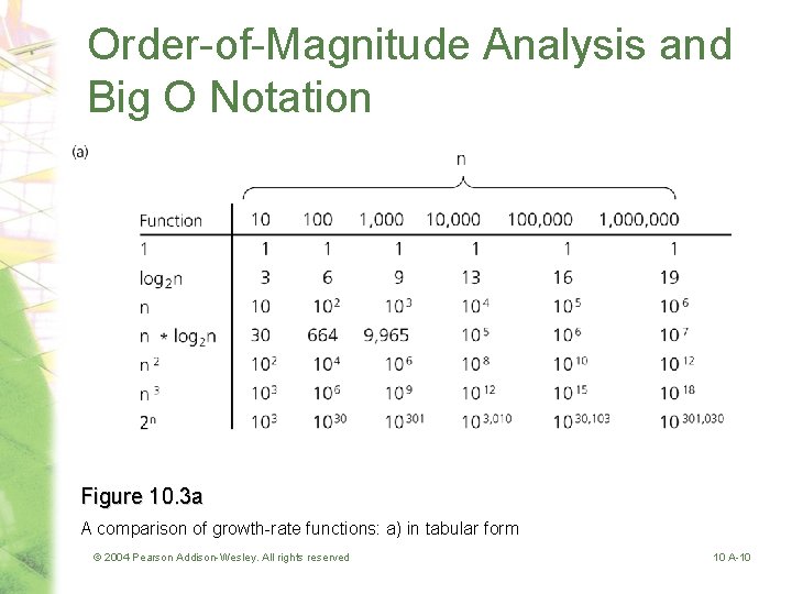
Order-of-Magnitude Analysis and Big O Notation Figure 10. 3 a A comparison of growth-rate functions: a) in tabular form © 2004 Pearson Addison-Wesley. All rights reserved 10 A-10

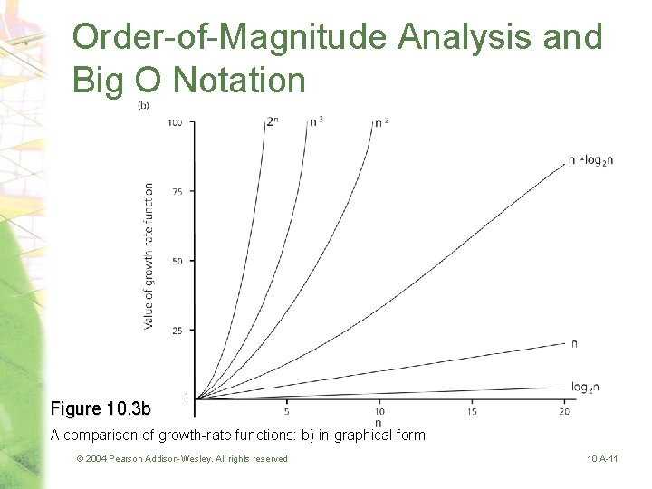
Order-of-Magnitude Analysis and Big O Notation Figure 10. 3 b A comparison of growth-rate functions: b) in graphical form © 2004 Pearson Addison-Wesley. All rights reserved 10 A-11

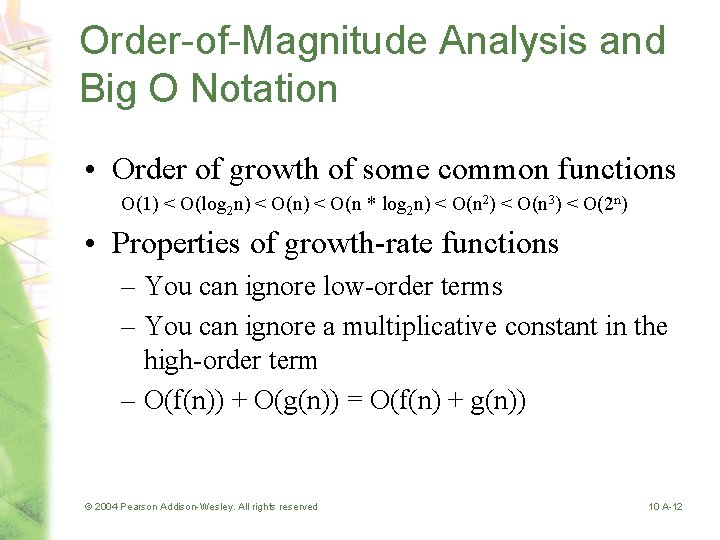
Order-of-Magnitude Analysis and Big O Notation • Order of growth of some common functions O(1) < O(log 2 n) < O(n * log 2 n) < O(n 2) < O(n 3) < O(2 n) • Properties of growth-rate functions – You can ignore low-order terms – You can ignore a multiplicative constant in the high-order term – O(f(n)) + O(g(n)) = O(f(n) + g(n)) © 2004 Pearson Addison-Wesley. All rights reserved 10 A-12

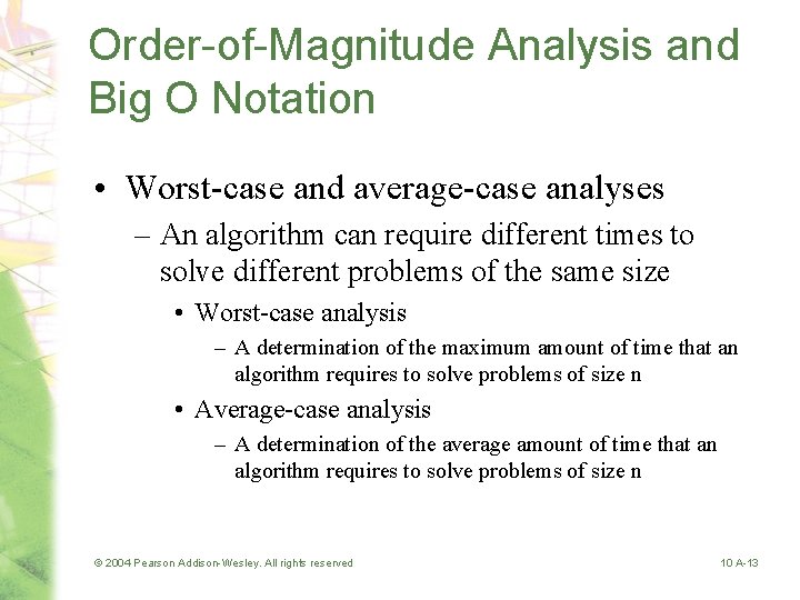
Order-of-Magnitude Analysis and Big O Notation • Worst-case and average-case analyses – An algorithm can require different times to solve different problems of the same size • Worst-case analysis – A determination of the maximum amount of time that an algorithm requires to solve problems of size n • Average-case analysis – A determination of the average amount of time that an algorithm requires to solve problems of size n © 2004 Pearson Addison-Wesley. All rights reserved 10 A-13

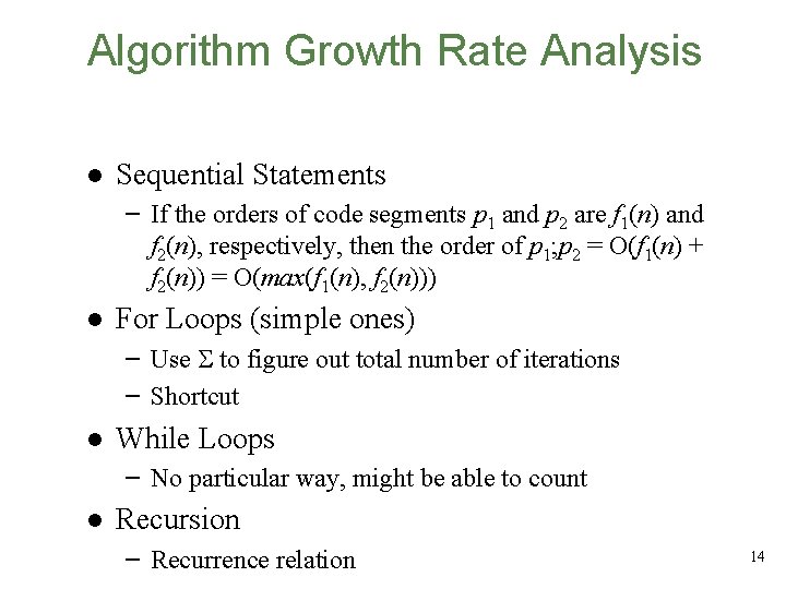
Algorithm Growth Rate Analysis l Sequential Statements – If the orders of code segments p 1 and p 2 are f 1(n) and f 2(n), respectively, then the order of p 1; p 2 = O(f 1(n) + f 2(n)) = O(max(f 1(n), f 2(n))) l For Loops (simple ones) – Use to figure out total number of iterations – Shortcut l While Loops – No particular way, might be able to count l Recursion – Recurrence relation 14

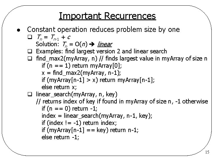
Important Recurrences l Constant operation reduces problem size by one q Tn = Tn-1 + c Solution: Tn = O(n) linear q Examples: find largest version 2 and linear search q find_max 2(my. Array, n) // finds largest value in my. Array of size n if (n == 1) return my. Array[0]; x = find_max 2(my. Array, n-1); if (my. Array[n-1] > x) return my. Array[n-1]; else return x; q linear_search(my. Array, n, key) // returns index of key if found in my. Array of size n, -1 otherwise if (n == 0) return -1; index = linear_search(my. Array, n-1, key); if (index != -1) return index; if (my. Array[n-1] == key) return n-1; else return -1; 15

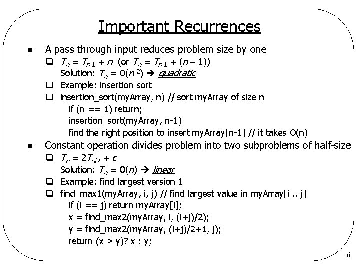
Important Recurrences l A pass through input reduces problem size by one q Tn = Tn-1 + n (or Tn = Tn-1 + (n – 1)) Solution: Tn = O(n 2) quadratic q Example: insertion sort q insertion_sort(my. Array, n) // sort my. Array of size n if (n == 1) return; insertion_sort(my. Array, n-1) find the right position to insert my. Array[n-1] // it takes O(n) l Constant operation divides problem into two subproblems of half-size q Tn = 2 Tn/2 + c Solution: Tn = O(n) linear q Example: find largest version 1 q find_max 1(my. Array, i, j) // find largest value in my. Array[i. . j] if (i == j) return my. Array[i]; x = find_max 2(my. Array, i, (i+j)/2); y = find_max 2(my. Array, (i+j)/2+1, j); return (x > y)? x : y; 16

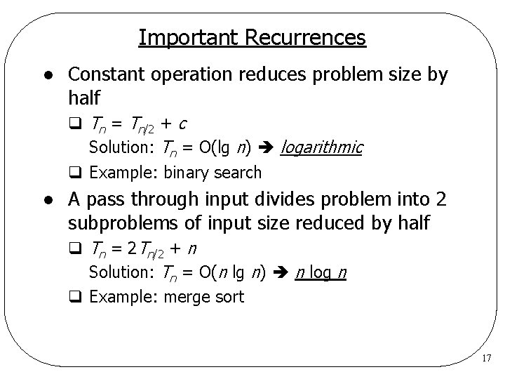
Important Recurrences l Constant operation reduces problem size by half q Tn = Tn/2 + c Solution: Tn = O(lg n) logarithmic q Example: binary search l A pass through input divides problem into 2 subproblems of input size reduced by half q Tn = 2 Tn/2 + n Solution: Tn = O(n lg n) n log n q Example: merge sort 17

Keeping Your Perspective • Throughout the course of an analysis, keep in mind that you are interested only in significant differences in efficiency • When choosing an ADT’s implementation, consider how frequently particular ADT operations occur in a given application • Some seldom-used but critical operations must be efficient © 2004 Pearson Addison-Wesley. All rights reserved 10 A-18

Keeping Your Perspective • If the problem size is always small, you can probably ignore an algorithm’s efficiency • Weigh the trade-offs between an algorithm’s time requirements and its memory requirements • Compare algorithms for both style and efficiency • Order-of-magnitude analysis focuses on large problems © 2004 Pearson Addison-Wesley. All rights reserved 10 A-19

The Efficiency of Searching Algorithms • Sequential search – Strategy • Look at each item in the data collection in turn, beginning with the first one • Stop when – You find the desired item – You reach the end of the data collection © 2004 Pearson Addison-Wesley. All rights reserved 10 A-20

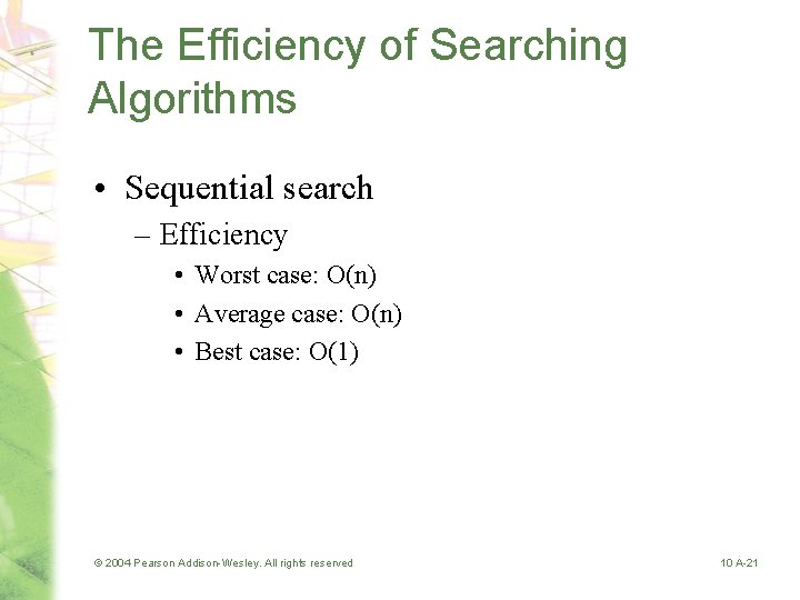
The Efficiency of Searching Algorithms • Sequential search – Efficiency • Worst case: O(n) • Average case: O(n) • Best case: O(1) © 2004 Pearson Addison-Wesley. All rights reserved 10 A-21

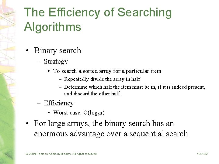
The Efficiency of Searching Algorithms • Binary search – Strategy • To search a sorted array for a particular item – Repeatedly divide the array in half – Determine which half the item must be in, if it is indeed present, and discard the other half – Efficiency • Worst case: O(log 2 n) • For large arrays, the binary search has an enormous advantage over a sequential search © 2004 Pearson Addison-Wesley. All rights reserved 10 A-22