Chapter 3 Image processing and computer vision Edge

Chapter 3: Image processing and computer vision Edge detection and image filtering by Prof. K. H. Wong, Computer Science and Engineering Dept. CUHK khwong@cse. cuhk. edu. hk Tutorial for CMSC 5711 : Edge v 0. 1 a 1

You will learn • Introduction: Edge detection by differentiation and threshold • Convolution math tool • Edge mask : edge detection by convolution (e. g. Sobel) • Image Filtering: smoothing, high pass etc. • Laplacian method : 2 nd order derivative method. • Laplacian of Gaussian : LOG smoothing and edge detection together • Canny Edge Detection: Most popular method Tutorial for CMSC 5711 : Edge v 0. 1 a 2

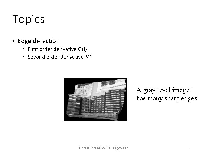
Topics • Edge detection • First order derivative G(I) • Second order derivative 2 I A gray level image I has many sharp edges Tutorial for CMSC 5711 : Edge v 0. 1 a 3

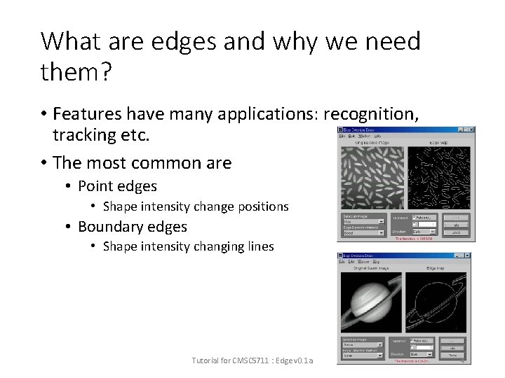
What are edges and why we need them? • Features have many applications: recognition, tracking etc. • The most common are • Point edges • Shape intensity change positions • Boundary edges • Shape intensity changing lines Tutorial for CMSC 5711 : Edge v 0. 1 a 4

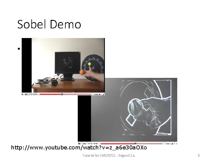
Sobel Demo • http: //www. youtube. com/watch? v=z_a 6 e 30 a. OXo Tutorial for CMSC 5711 : Edge v 0. 1 a 5

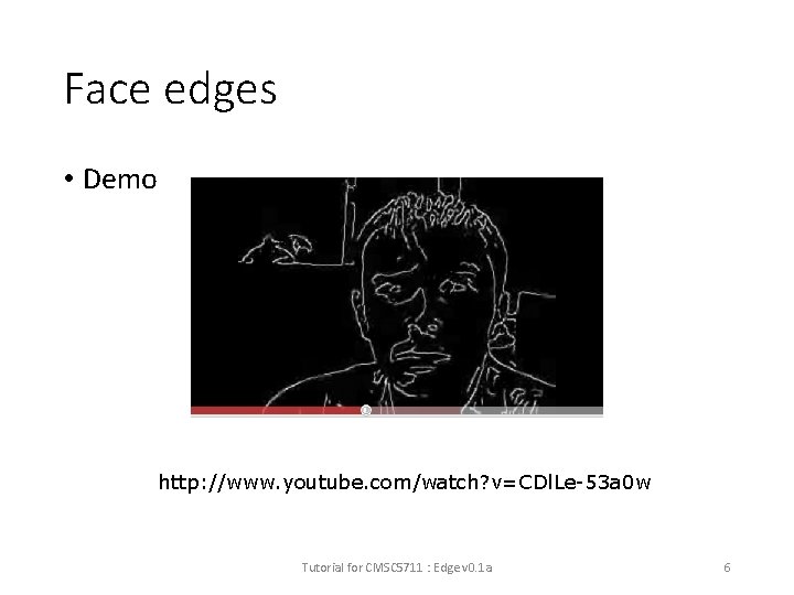
Face edges • Demo http: //www. youtube. com/watch? v=CDl. Le-53 a 0 w Tutorial for CMSC 5711 : Edge v 0. 1 a 6

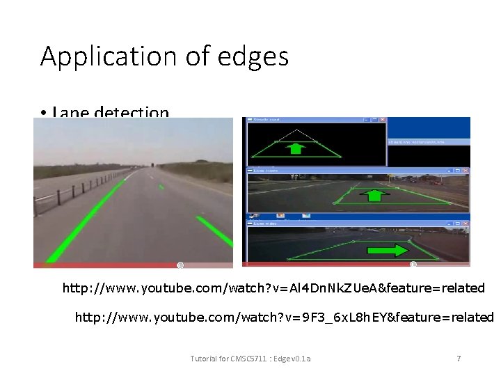
Application of edges • Lane detection http: //www. youtube. com/watch? v=Al 4 Dn. Nk. ZUe. A&feature=related http: //www. youtube. com/watch? v=9 F 3_6 x. L 8 h. EY&feature=related Tutorial for CMSC 5711 : Edge v 0. 1 a 7

How to obtained edges? • Use gradient G of intensity [I(x, y)] change, two methods • First order gradient I(x, y+1) I(x+1, y+1) I(x, y) I(x+1, y) I(x, y) • I(x, y) is an edge if y • Second order gradient (Laplacian operator) • I(x, y) is an edge if Tutorial for CMSC 5711 : Edge v 0. 1 a x 8

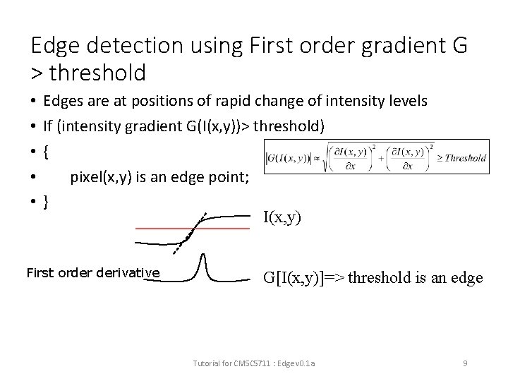
Edge detection using First order gradient G > threshold • • • Edges are at positions of rapid change of intensity levels If (intensity gradient G(I(x, y))> threshold) { pixel(x, y) is an edge point; } I(x, y) First order derivative G[I(x, y)]=> threshold is an edge Tutorial for CMSC 5711 : Edge v 0. 1 a 9

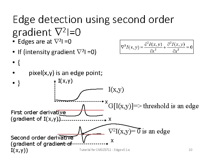
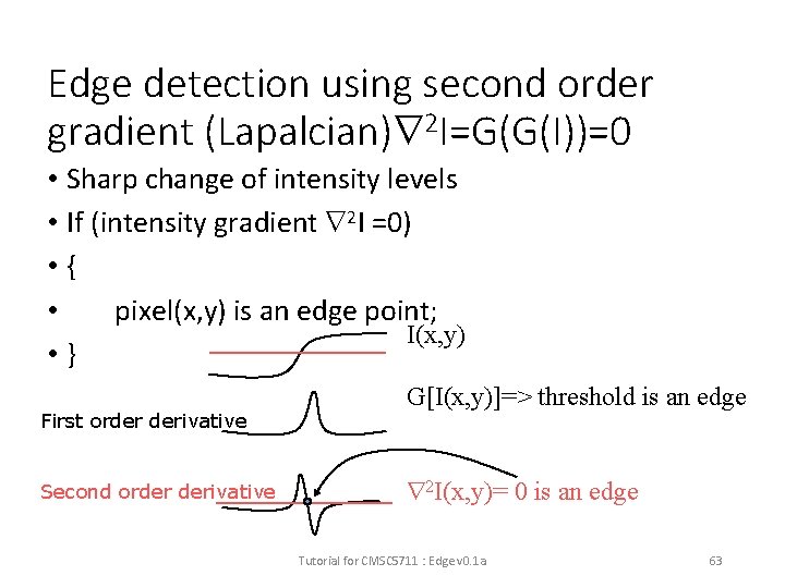
Edge detection using second order gradient 2 I=0 • • • Edges are at 2 I =0 If (intensity gradient 2 I =0) { pixel(x, y) is an edge point; I(x, y) } I(x, y) x First order derivative (gradient of I(x, y)) Second order derivative (gradient of I(x, y)) G[I(x, y)]=> threshold is an edge x 2 I(x, y)= 0 is an edge x Tutorial for CMSC 5711 : Edge v 0. 1 a 10

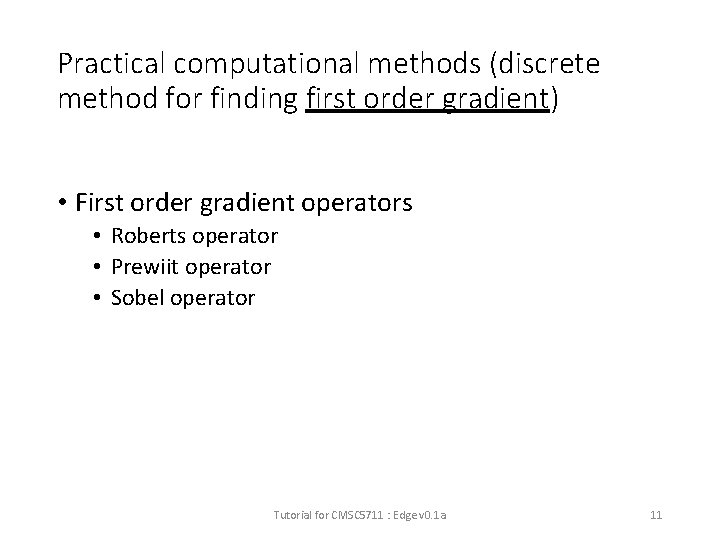
Practical computational methods (discrete method for finding first order gradient) • First order gradient operators • Roberts operator • Prewiit operator • Sobel operator Tutorial for CMSC 5711 : Edge v 0. 1 a 11

Convolution method • Convolution is an important and popular technique in signal processing • Edges can found by convoluting an image with a mask Tutorial for CMSC 5711 : Edge v 0. 1 a 12

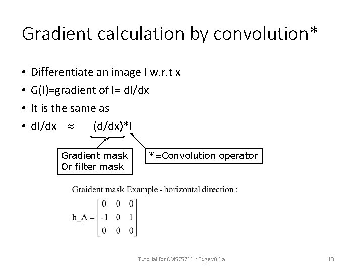
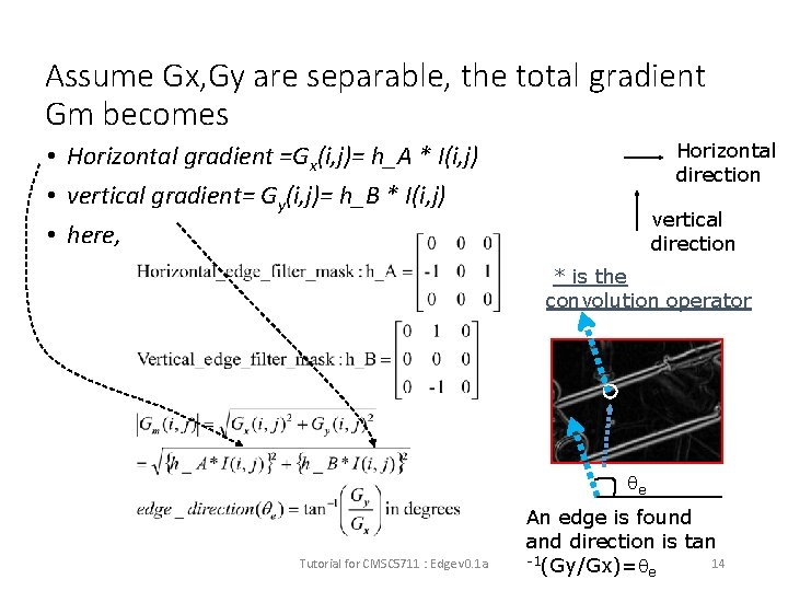
Gradient calculation by convolution* • • Differentiate an image I w. r. t x G(I)=gradient of I= d. I/dx It is the same as d. I/dx (d/dx)*I Gradient mask Or filter mask *=Convolution operator Tutorial for CMSC 5711 : Edge v 0. 1 a 13

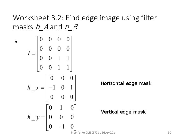
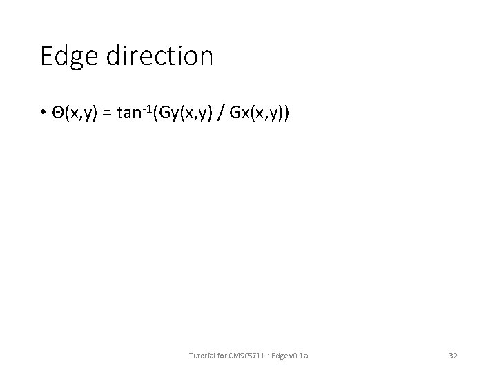
Assume Gx, Gy are separable, the total gradient Gm becomes Horizontal direction • Horizontal gradient =Gx(i, j)= h_A * I(i, j) • vertical gradient= Gy(i, j)= h_B * I(i, j) • here, vertical direction * is the convolution operator e Tutorial for CMSC 5711 : Edge v 0. 1 a An edge is found and direction is tan -1(Gy/Gx)= 14 e

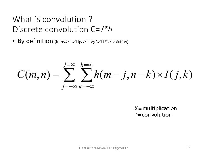
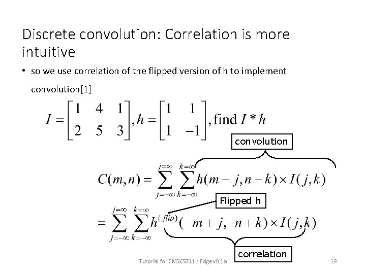
What is convolution ? Discrete convolution C=I*h • By definition (http: //en. wikipedia. org/wiki/Convolution) X=multiplication *=convolution Tutorial for CMSC 5711 : Edge v 0. 1 a 15

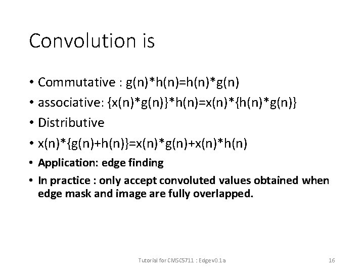
Convolution is • Commutative : g(n)*h(n)=h(n)*g(n) • associative: {x(n)*g(n)}*h(n)=x(n)*{h(n)*g(n)} • Distributive • x(n)*{g(n)+h(n)}=x(n)*g(n)+x(n)*h(n) • Application: edge finding • In practice : only accept convoluted values obtained when edge mask and image are fully overlapped. Tutorial for CMSC 5711 : Edge v 0. 1 a 16

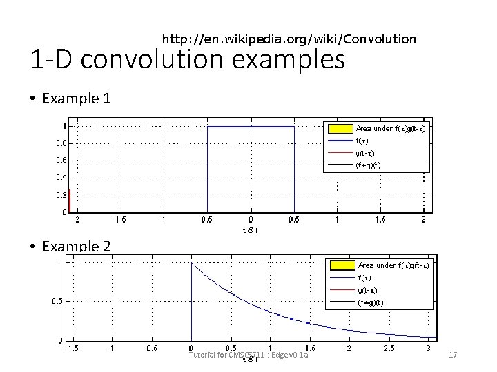
http: //en. wikipedia. org/wiki/Convolution 1 -D convolution examples • Example 1 • Example 2 Tutorial for CMSC 5711 : Edge v 0. 1 a 17

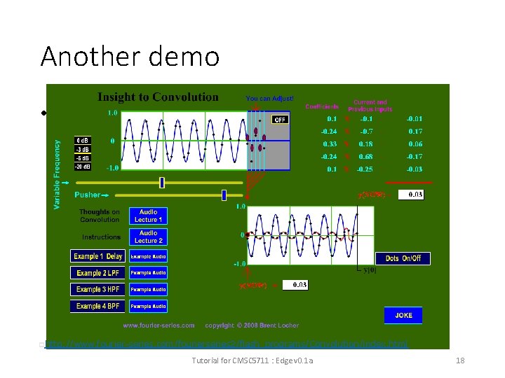
Another demo • phttp: //www. fourier-series. com/fourierseries 2/flash_programs/Convolution/index. html Tutorial for CMSC 5711 : Edge v 0. 1 a 18

Discrete convolution: Correlation is more intuitive • so we use correlation of the flipped version of h to implement convolution[1] convolution Flipped h Tutorial for CMSC 5711 : Edge v 0. 1 a correlation 19

Matlab (octave) code for convolution • • • I=[1 4 1; 2 5 3] h=[1 1 ; 1 -1] conv 2(I, h) pause disp('It is the same as the following'); conv 2(h, I) pause disp('It is the same as the following'); xcorr 2(I, fliplr(flipud(h))) Tutorial for CMSC 5711 : Edge v 0. 1 a 20

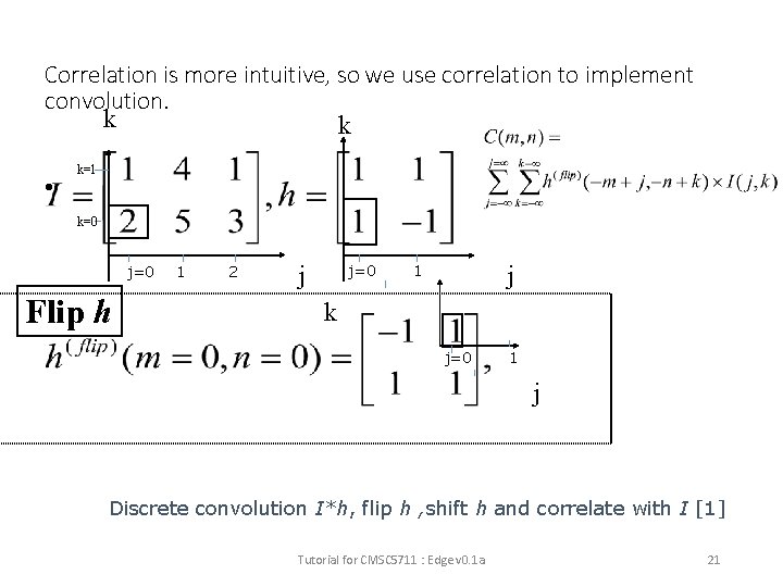
Correlation is more intuitive, so we use correlation to implement convolution. k k • k=1 k=0 j=0 Flip h 1 2 j j=0 j 1 k j=0 1 j Discrete convolution I*h, flip h , shift h and correlate with I [1] Tutorial for CMSC 5711 : Edge v 0. 1 a 21

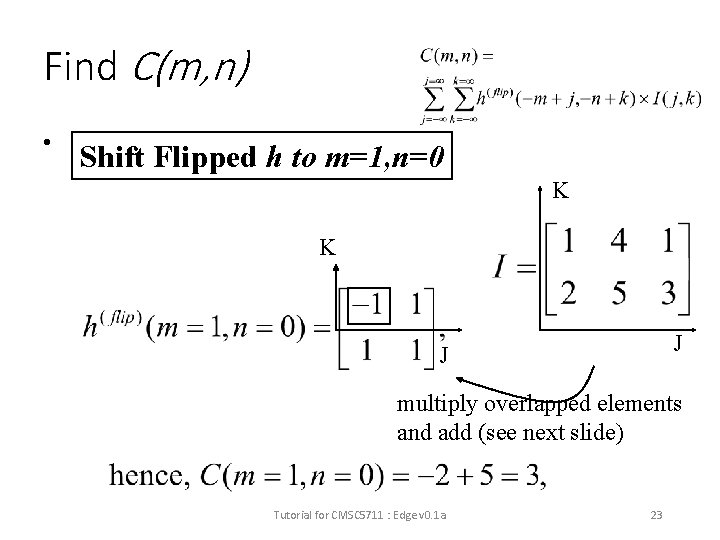
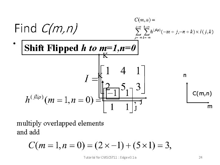
Discrete convolution I*h, flip h , shift h and correlate with I [1] k k • n j j=0 j 1 Flip h: is like this after the flip k and no shift (m=0, n=0) j Shift Flipped h to m=1, n=0 k j Tutorial for CMSC 5711 : Edge v 0. 1 a C(m, n) m The trick: I(j=0, k=0) needs to multiply to h(flip)(-m+0, -n+0), since m=1, n=0, so we shift the h(flip) pattern 1 -bit to the right so we just multiply overlapped elements of I and h(flip). Similarly, we do the same for all m, n values 22

Find C(m, n) • Shift Flipped h to m=1, n=0 K K J J multiply overlapped elements and add (see next slide) Tutorial for CMSC 5711 : Edge v 0. 1 a 23

Find C(m, n) • Shift Flipped h to m=1, n=0 K K n C(m, n) J J m multiply overlapped elements and add Tutorial for CMSC 5711 : Edge v 0. 1 a 24

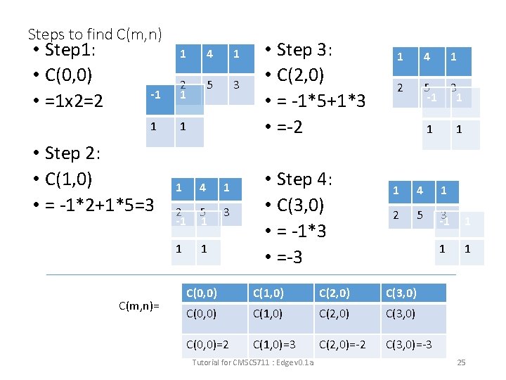
Steps to find C(m, n) • Step 1: • C(0, 0) • =1 x 2=2 1 4 1 -1 2 1 5 3 1 1 • Step 2: • C(1, 0) • = -1*2+1*5=3 C(m, n)= 1 4 1 2 -1 5 1 3 1 1 • Step 3: • C(2, 0) • = -1*5+1*3 • =-2 • Step 4: • C(3, 0) • = -1*3 • =-3 1 4 1 2 5 -1 3 1 1 4 1 2 5 3 -1 1 C(0, 0) C(1, 0) C(2, 0) C(3, 0) C(0, 0)=2 C(1, 0)=3 C(2, 0)=-2 C(3, 0)=-3 Tutorial for CMSC 5711 : Edge v 0. 1 a 25

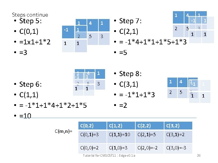
Steps continue • • Step 5: C(0, 1) =1 x 1+1*2 =3 -1 1 2 1 1 -1 2 1 4 1 5 3 4 1 5 1 Step 6: C(1, 1) = -1*1+1*4+1*2+1*5 =10 C(m, n)= 1 3 1 4 1 • • -1 Step 7: 2 5 3 C(2, 1) 1 = -1*4+1*1+1*5+1*3 =5 • • Step 8: C(3, 1) = -1*1+1*3 =2 1 4 2 5 C(0, 2) C(1, 2) C(2, 2) C(3, 2) C(0, 1)=3 C(1, 1)=10 C(2, 1)=5 C(3, 1)=2 C(0, 0)=2 C(1, 0)=3 C(2, 0)=-2 C(3, 0)=-3 Tutorial for CMSC 5711 : Edge v 0. 1 a 1 -1 3 1 1 1 26

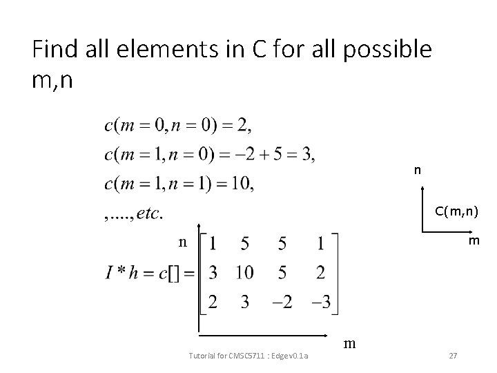
Find all elements in C for all possible m, n n C(m, n) n m Tutorial for CMSC 5711 : Edge v 0. 1 a m 27

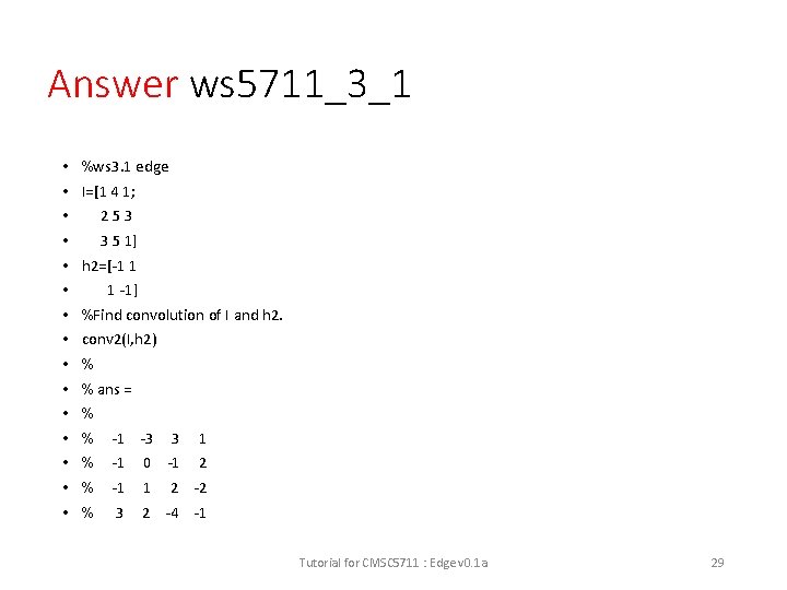
Worksheet 3. 1 • I=[1 4 1; • 253 • 3 5 1] • h 2=[-1 1 • 1 -1] • Find convolution of I and h 2. Tutorial for CMSC 5711 : Edge v 0. 1 a 28

Answer ws 5711_3_1 • • • • %ws 3. 1 edge I=[1 4 1; 253 3 5 1] h 2=[-1 1 1 -1] %Find convolution of I and h 2. conv 2(I, h 2) % % ans = % % -1 -3 3 1 % -1 0 -1 2 % -1 1 % 3 2 -4 -1 2 -2 Tutorial for CMSC 5711 : Edge v 0. 1 a 29

Worksheet 3. 2: Find edge image using filter masks h_A and h_B • Horizontal edge mask Vertical edge mask Tutorial for CMSC 5711 : Edge v 0. 1 a 30

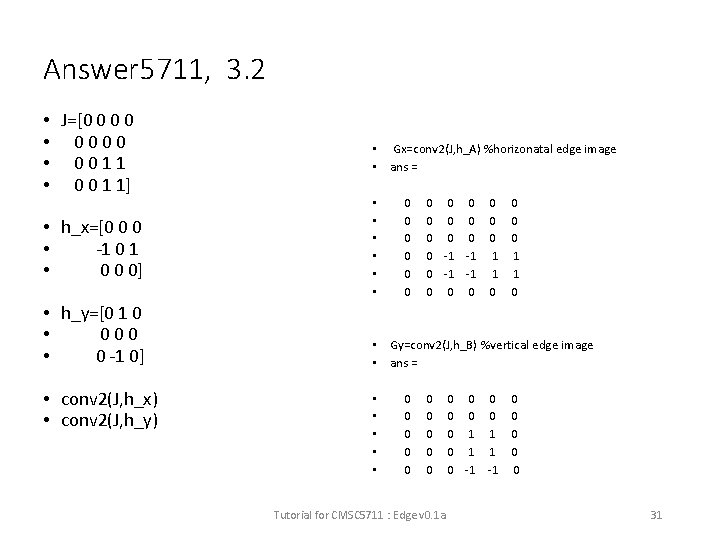
Answer 5711, 3. 2 • J=[0 0 • 0000 • 0011 • 0 0 1 1] • h_x=[0 0 0 • -1 0 1 • 0 0 0] • h_y=[0 1 0 • 000 • 0 -1 0] • conv 2(J, h_x) • conv 2(J, h_y) • Gx=conv 2(J, h_A) %horizonatal edge image • ans = • • • 0 0 0 0 0 -1 -1 1 0 0 0 0 1 1 0 • Gy=conv 2(J, h_B) %vertical edge image • ans = • • • 0 0 0 0 0 Tutorial for CMSC 5711 : Edge v 0. 1 a 0 0 0 0 1 1 0 -1 -1 0 0 0 31

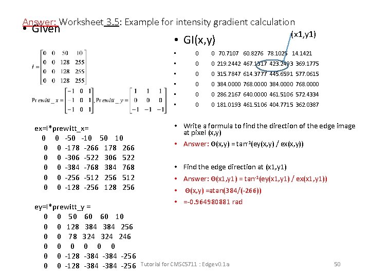
Edge direction • Θ(x, y) = tan-1(Gy(x, y) / Gx(x, y)) Tutorial for CMSC 5711 : Edge v 0. 1 a 32

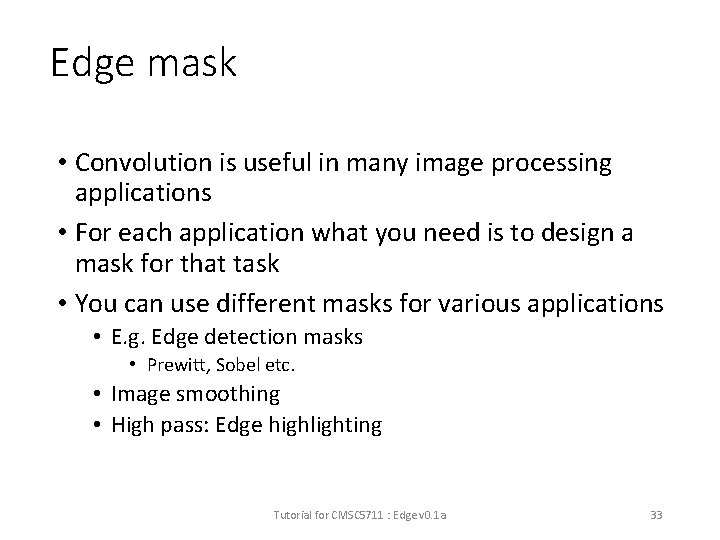
Edge mask • Convolution is useful in many image processing applications • For each application what you need is to design a mask for that task • You can use different masks for various applications • E. g. Edge detection masks • Prewitt, Sobel etc. • Image smoothing • High pass: Edge highlighting Tutorial for CMSC 5711 : Edge v 0. 1 a 33

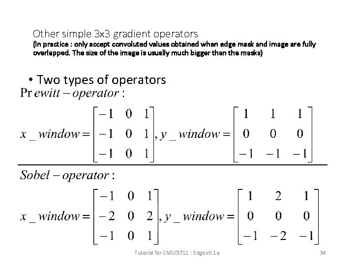
Other simple 3 x 3 gradient operators (In practice : only accept convoluted values obtained when edge mask and image are fully overlapped. The size of the image is usually much bigger than the masks) • Two types of operators Tutorial for CMSC 5711 : Edge v 0. 1 a 34

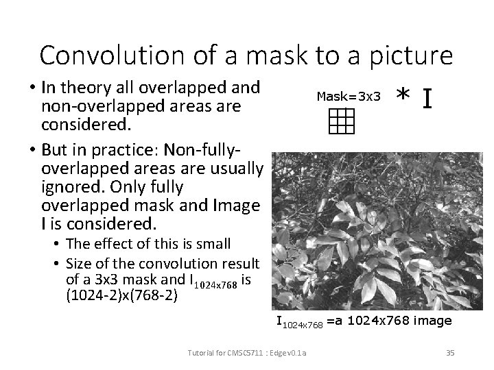
Convolution of a mask to a picture • In theory all overlapped and non-overlapped areas are considered. • But in practice: Non-fullyoverlapped areas are usually ignored. Only fully overlapped mask and Image I is considered. Mask=3 x 3 *I • The effect of this is small • Size of the convolution result of a 3 x 3 mask and I 1024 x 768 is (1024 -2)x(768 -2) I 1024 x 768 =a 1024 x 768 image Tutorial for CMSC 5711 : Edge v 0. 1 a 35

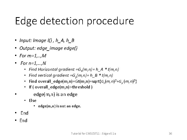
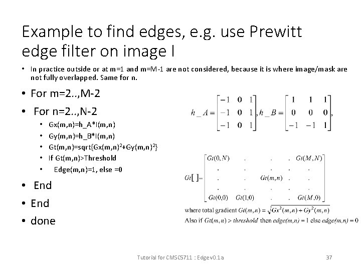
Edge detection procedure • • Input: Image I() , h_A, h_B Output: edge_image edge() For m=1, . . , M For n=1, …, N • • Find Horizontal gradient =Gx(m, n)= h_A * I(m, n) Find vertical gradient =Gy(m, n)= h_B * I(m, n) Find overall_edge(m, n)=Gt(m, n)=sqrt{Gx(m, n)2+Gy (m, n)2} If ( overall_edge(m, n)>threshold ) edge(m, n) is an edge • • Else • edge(m, n) is not an edge. • End Tutorial for CMSC 5711 : Edge v 0. 1 a 36

Example to find edges, e. g. use Prewitt edge filter on image I • In practice outside or at m=1 and m=M-1 are not considered, because it is where image/mask are not fully overlapped. Same for n. • For m=2. . , M-2 • For n=2. . , N-2 • • • Gx(m, n)=h_A*I(m, n) Gy(m, n)=h_B*I(m, n) Gt(m, n)=sqrt{Gx(m, n)2+Gy(m, n)2} If Gt(m, n)>Threshold Edge(m, n)=1, else =0 • End • done Tutorial for CMSC 5711 : Edge v 0. 1 a 37

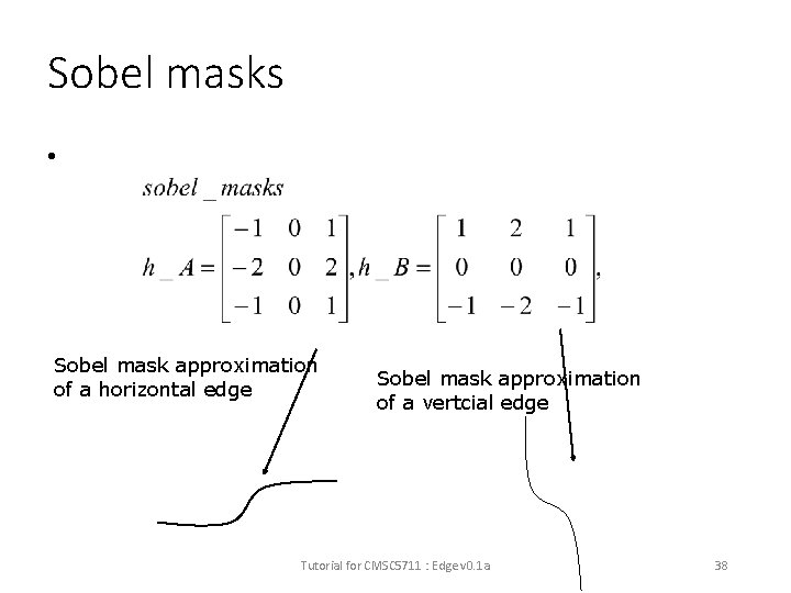
Sobel masks • Sobel mask approximation of a horizontal edge Sobel mask approximation of a vertcial edge Tutorial for CMSC 5711 : Edge v 0. 1 a 38

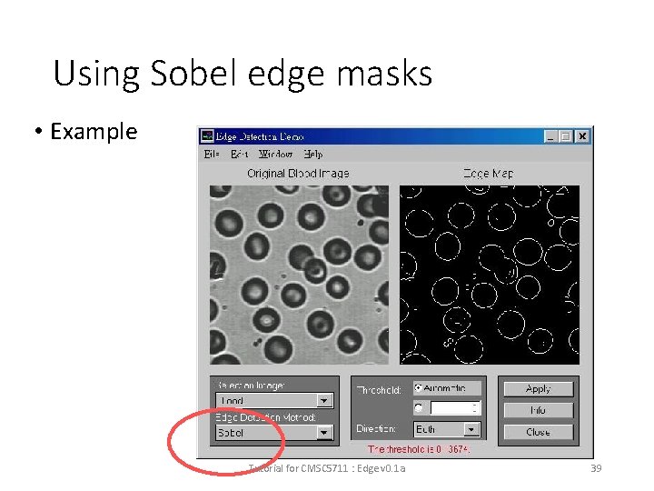
Using Sobel edge masks • Example Tutorial for CMSC 5711 : Edge v 0. 1 a 39

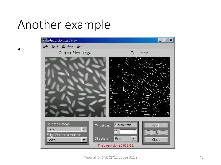
Another example • Tutorial for CMSC 5711 : Edge v 0. 1 a 40

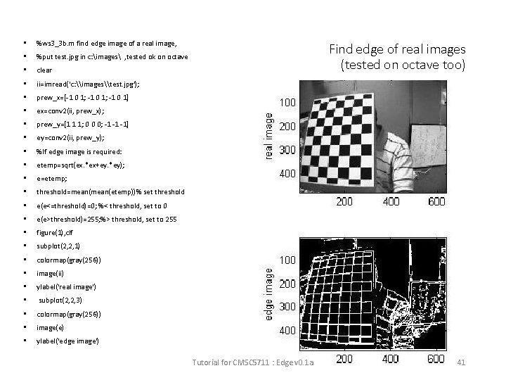
• %ws 3_3 b. m find edge image of a real image, • %put test. jpg in c: images , tested ok on octave • clear • ii=imread('c: \images\test. jpg'); • prew_x=[-1 0 1; -1 0 1] • ex=conv 2(ii, prew_x); • prew_y=[1 1 1; 0 0 0; -1 -1 -1] • ey=conv 2(ii, prew_y); • %If edge image is required: • etemp=sqrt(ex. *ex+ey. *ey); • e=etemp; • threshold=mean(etemp))% set threshold • e(e<=threshold)=0; %< threshold, set to 0 • e(e>threshold)=255; %> threshold, set to 255 • figure(1), clf • subplot(2, 2, 1) • colormap(gray(256)) • image(ii) • ylabel('real image') • subplot(2, 2, 3) • colormap(gray(256)) • image(e) • ylabel('edge image') Find edge of real images (tested on octave too) Tutorial for CMSC 5711 : Edge v 0. 1 a 41

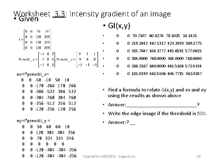
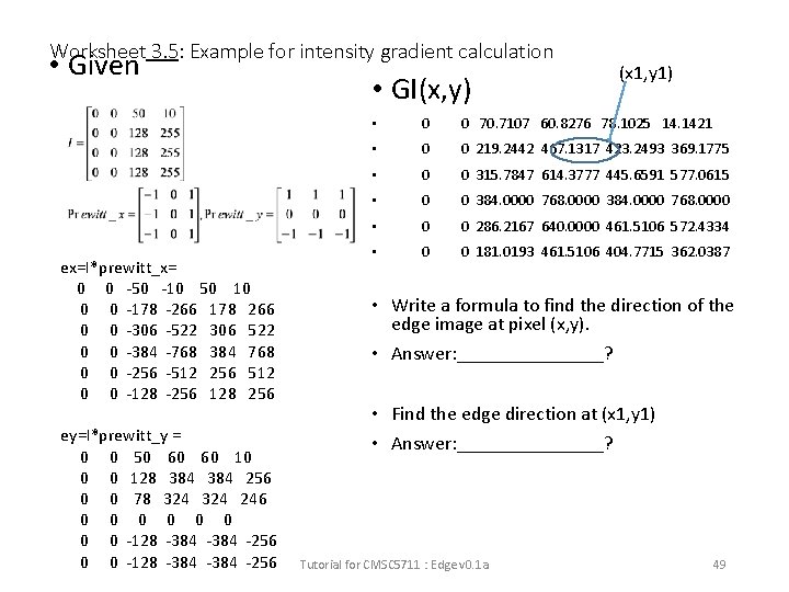
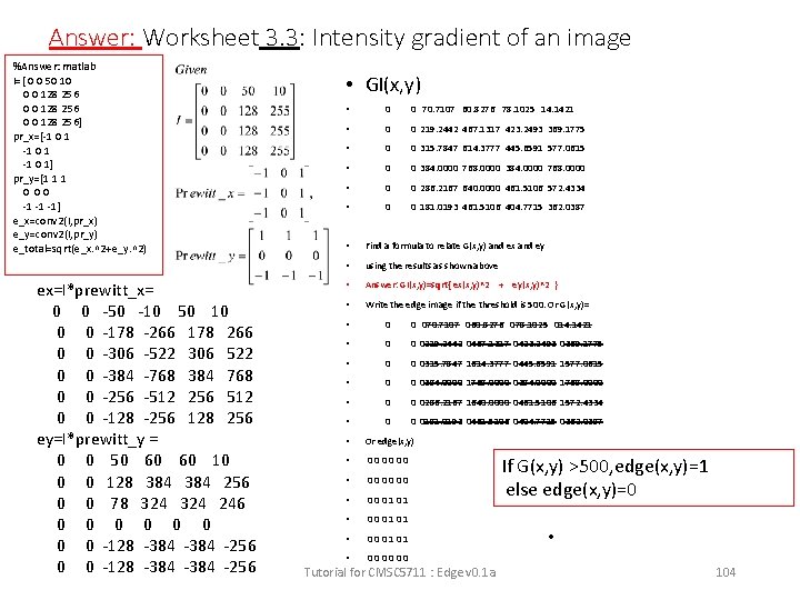
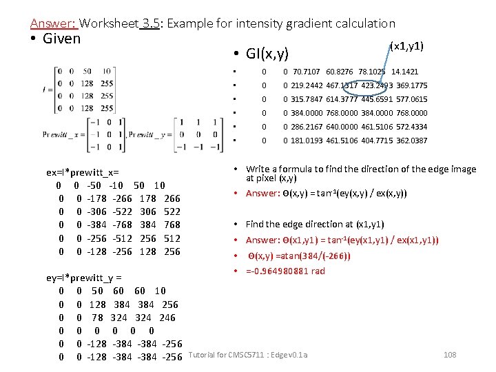
Worksheet 3. 3: Intensity gradient of an image • Given • GI(x, y) • 0 0 70. 7107 60. 8276 78. 1025 14. 1421 • 0 0 219. 2442 467. 1317 423. 2493 369. 1775 • 0 0 315. 7847 614. 3777 445. 6591 577. 0615 • 0 0 384. 0000 768. 0000 • 0 0 286. 2167 640. 0000 461. 5106 572. 4334 ex=I*prewitt_x= 0 0 -50 -10 50 10 0 0 -178 -266 178 266 0 0 -306 -522 306 522 0 0 -384 -768 384 768 0 0 -256 -512 256 512 0 0 -128 -256 128 256 • 0 0 181. 0193 461. 5106 404. 7715 362. 0387 ey=I*prewitt_y = 0 0 50 60 60 10 0 0 128 384 256 0 0 78 324 246 0 0 0 0 -128 -384 -256 • Answer: ? __ • Find a formula to relate G(x, y) and ex and ey using the results as shown above • Answer: _____________? • Write the edge image if the threshold is 500. Tutorial for CMSC 5711 : Edge v 0. 1 a 42

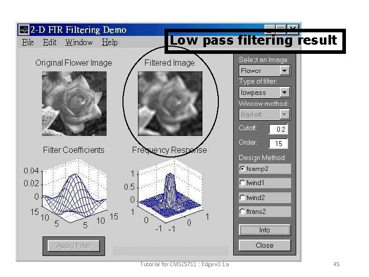
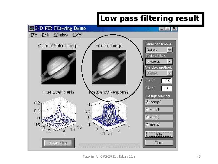
Image filtering You may design a mask for Low pass filtering (smoothing filter) Low pass Tutorial for CMSC 5711 : Edge v 0. 1 a 43

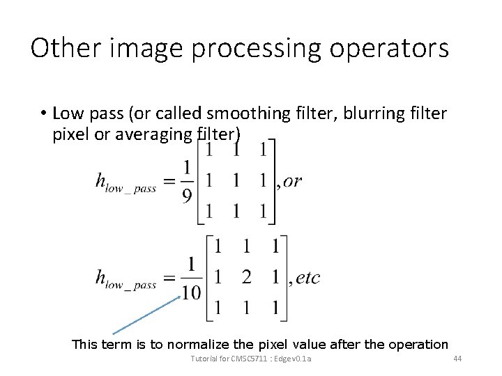
Other image processing operators • Low pass (or called smoothing filter, blurring filter pixel or averaging filter) This term is to normalize the pixel value after the operation Tutorial for CMSC 5711 : Edge v 0. 1 a 44

Low pass filtering result Tutorial for CMSC 5711 : Edge v 0. 1 a 45

Low pass filtering result Tutorial for CMSC 5711 : Edge v 0. 1 a 46

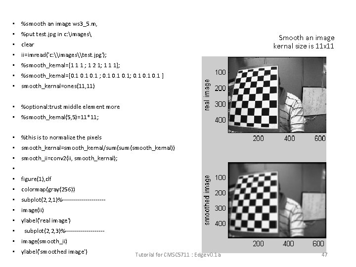
• %smooth an image ws 3_5. m, • %put test. jpg in c: images Smooth an image kernal size is 11 x 11 • clear • ii=imread('c: \images\test. jpg'); • %smooth_kernal=[1 1 1 ; 1 2 1; 1 1 1]; • %smooth_kernal=[0. 1 ; 0. 1 0. 1 ] • smooth_kernal=ones(11, 11) • %optional: trust middle element more • %smooth_kernal(5, 5)=11*11; • %this is to normalize the pixels • smooth_kernal=smooth_kernal/sum(smooth_kernal)) • smooth_ii=conv 2(ii, smooth_kernal); • • figure(1), clf • colormap(gray(256)) • subplot(2, 2, 1)%----------- • image(ii) • ylabel('real image') • subplot(2, 2, 3)%---------- • image(smooth_ii) • ylabel('smoothed image') Tutorial for CMSC 5711 : Edge v 0. 1 a 47

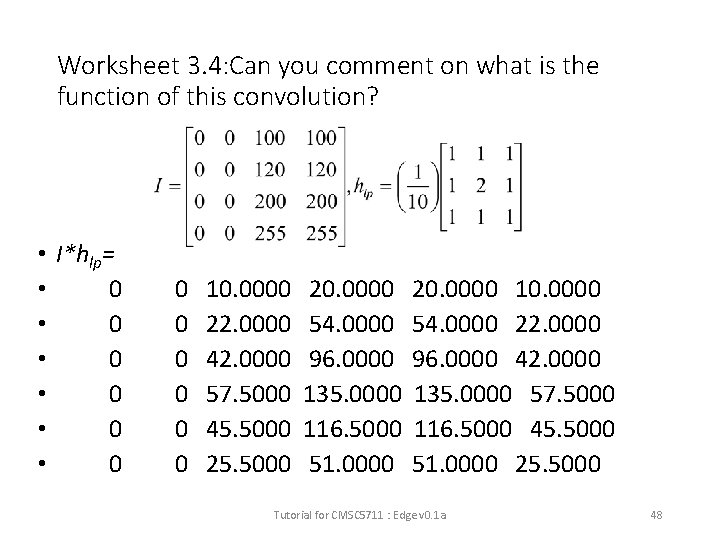
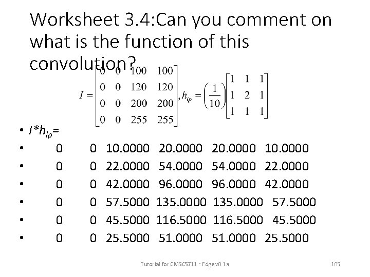
Worksheet 3. 4: Can you comment on what is the function of this convolution? • I*hlp= • 0 • 0 • 0 0 0 0 10. 0000 22. 0000 42. 0000 57. 5000 45. 5000 20. 0000 54. 0000 96. 0000 135. 0000 116. 5000 51. 0000 20. 0000 10. 0000 54. 0000 22. 0000 96. 0000 42. 0000 135. 0000 57. 5000 116. 5000 45. 5000 51. 0000 25. 5000 Tutorial for CMSC 5711 : Edge v 0. 1 a 48

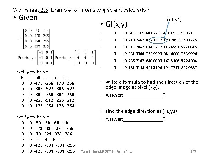
Worksheet 3. 5: Example for intensity gradient calculation • Given ex=I*prewitt_x= 0 0 -50 -10 50 10 0 0 -178 -266 178 266 0 0 -306 -522 306 522 0 0 -384 -768 384 768 0 0 -256 -512 256 512 0 0 -128 -256 128 256 ey=I*prewitt_y = 0 0 50 60 60 10 0 0 128 384 256 0 0 78 324 246 0 0 0 0 -128 -384 -256 • GI(x, y) (x 1, y 1) • 0 0 70. 7107 60. 8276 78. 1025 14. 1421 • 0 0 219. 2442 467. 1317 423. 2493 369. 1775 • 0 0 315. 7847 614. 3777 445. 6591 577. 0615 • 0 0 384. 0000 768. 0000 • 0 0 286. 2167 640. 0000 461. 5106 572. 4334 • 0 0 181. 0193 461. 5106 404. 7715 362. 0387 • Write a formula to find the direction of the edge image at pixel (x, y). • Answer: ________? • Find the edge direction at (x 1, y 1) • Answer: ________? Tutorial for CMSC 5711 : Edge v 0. 1 a 49

Answer: Worksheet 3. 5: Example for intensity gradient calculation • Given ex=I*prewitt_x= 0 0 -50 -10 50 10 0 0 -178 -266 178 266 0 0 -306 -522 306 522 0 0 -384 -768 384 768 0 0 -256 -512 256 512 0 0 -128 -256 128 256 ey=I*prewitt_y = 0 0 50 60 60 10 0 0 128 384 256 0 0 78 324 246 0 0 0 0 -128 -384 -256 • GI(x, y) (x 1, y 1) • 0 0 70. 7107 60. 8276 78. 1025 14. 1421 • 0 0 219. 2442 467. 1317 423. 2493 369. 1775 • 0 0 315. 7847 614. 3777 445. 6591 577. 0615 • 0 0 384. 0000 768. 0000 • 0 0 286. 2167 640. 0000 461. 5106 572. 4334 • 0 0 181. 0193 461. 5106 404. 7715 362. 0387 • Write a formula to find the direction of the edge image at pixel (x, y) • Answer: Θ(x, y) = tan-1(ey(x, y) / ex(x, y)) • Find the edge direction at (x 1, y 1) • Answer: Θ(x 1, y 1) = tan-1(ey(x 1, y 1) / ex(x 1, y 1)) • Θ(x, y) =atan(384/(-266)) • =-0. 964980881 rad Tutorial for CMSC 5711 : Edge v 0. 1 a 50

A small summary • If you convolve an image I with an edge mask, you get an edge image. • If you convolve an image I with a smoothing mask, you get a smoothed image. Tutorial for CMSC 5711 : Edge v 0. 1 a 51

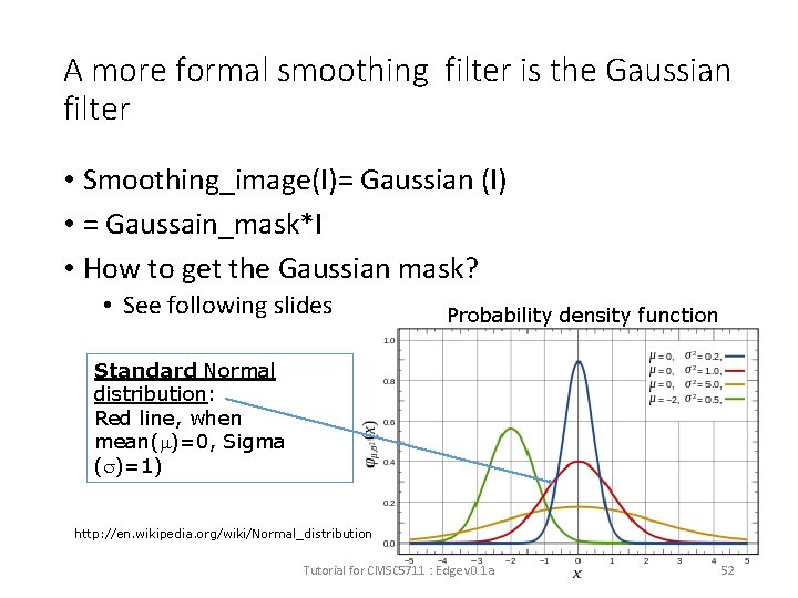
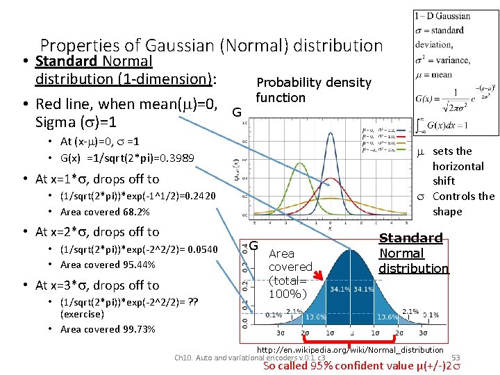
A more formal smoothing filter is the Gaussian filter • Smoothing_image(I)= Gaussian (I) • = Gaussain_mask*I • How to get the Gaussian mask? • See following slides Probability density function Standard Normal distribution: Red line, when mean( )=0, Sigma ( )=1) http: //en. wikipedia. org/wiki/Normal_distribution Tutorial for CMSC 5711 : Edge v 0. 1 a 52

Properties of Gaussian (Normal) distribution • Standard Normal distribution (1 -dimension): • Red line, when mean( )=0, Sigma ( )=1 G Probability density function • At (x- )=0, =1 • G(x) =1/sqrt(2*pi)=0. 3989 sets the horizontal shift Controls the shape • At x=1* , drops off to • (1/sqrt(2*pi))*exp(-1^1/2)=0. 2420 • Area covered 68. 2% • At x=2* , drops off to • (1/sqrt(2*pi))*exp(-2^2/2)= 0. 0540 • Area covered 95. 44% • At x=3* , drops off to • (1/sqrt(2*pi))*exp(-2^2/2)= ? ? (exercise) • Area covered 99. 73% G Area covered (total= 100%) Standard Normal distribution http: //en. wikipedia. org/wiki/Normal_distribution Ch 10. Auto and variational encoders v. 0. 1. c 3 53 So called 95% confident value µ(+/-)2

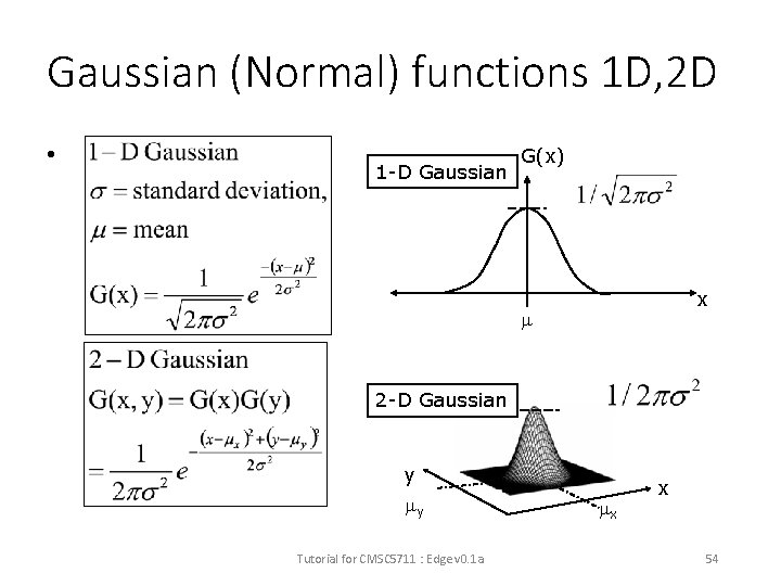
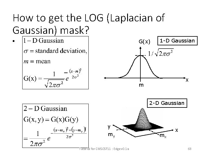
Gaussian (Normal) functions 1 D, 2 D • 1 -D Gaussian G(x) x 2 -D Gaussian y y Tutorial for CMSC 5711 : Edge v 0. 1 a x x 54

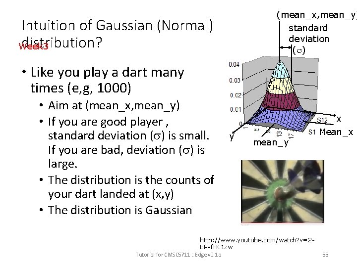
(mean_x, mean_y) Intuition of Gaussian (Normal) distribution? Week 3 standard deviation ( ) • Like you play a dart many times (e, g, 1000) • Aim at (mean_x, mean_y) • If you are good player , standard deviation ( ) is small. If you are bad, deviation ( ) is large. • The distribution is the counts of your dart landed at (x, y) • The distribution is Gaussian x y mean_y http: //www. youtube. com/watch? v=2 EPvf. FK 1 zw Tutorial for CMSC 5711 : Edge v 0. 1 a Mean_x 55

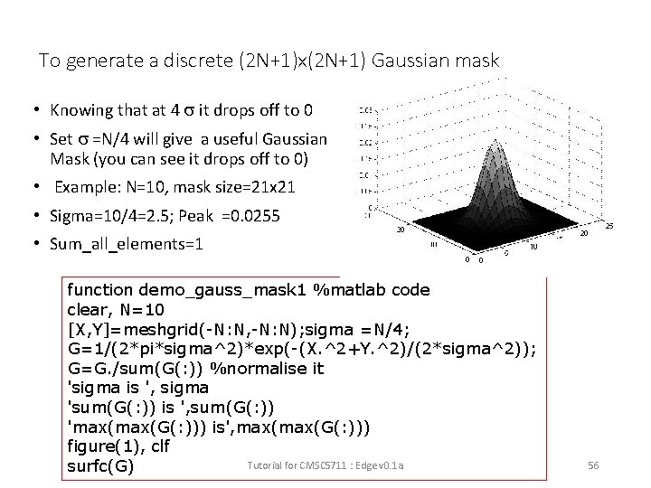
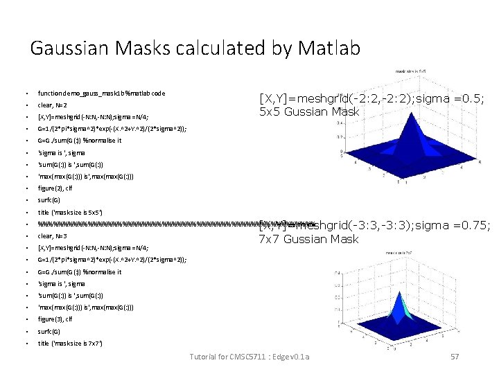
To generate a discrete (2 N+1)x(2 N+1) Gaussian mask • Knowing that at 4 it drops off to 0 • Set =N/4 will give a useful Gaussian Mask (you can see it drops off to 0) • Example: N=10, mask size=21 x 21 • Sigma=10/4=2. 5; Peak =0. 0255 • Sum_all_elements=1 function demo_gauss_mask 1 %matlab code clear, N=10 [X, Y]=meshgrid(-N: N, -N: N); sigma =N/4; G=1/(2*pi*sigma^2)*exp(-(X. ^2+Y. ^2)/(2*sigma^2)); G=G. /sum(G(: )) %normalise it 'sigma is ', sigma 'sum(G(: )) is ', sum(G(: )) 'max(G(: ))) is', max(G(: ))) figure(1), clf Tutorial for CMSC 5711 : Edge v 0. 1 a surfc(G) 56

Gaussian Masks calculated by Matlab • function demo_gauss_mask 1 b %matlab code • clear, N=2 • [X, Y]=meshgrid(-N: N, -N: N); sigma =N/4; • G=1/(2*pi*sigma^2)*exp(-(X. ^2+Y. ^2)/(2*sigma^2)); • G=G. /sum(G(: )) %normalise it • 'sigma is ', sigma • 'sum(G(: )) is ', sum(G(: )) • 'max(G(: ))) is', max(G(: ))) • figure(2), clf • surfc(G) • title ('mask size is 5 x 5') • %%%%%%%%%%%%%%%%%%%%%%%%%%%% • clear, N=3 • [X, Y]=meshgrid(-N: N, -N: N); sigma =N/4; • G=1/(2*pi*sigma^2)*exp(-(X. ^2+Y. ^2)/(2*sigma^2)); • G=G. /sum(G(: )) %normalise it • 'sigma is ', sigma • 'sum(G(: )) is ', sum(G(: )) • 'max(G(: ))) is', max(G(: ))) • figure(3), clf • surfc(G) • title ('mask size is 7 x 7') [X, Y]=meshgrid(-2: 2, -2: 2); sigma =0. 5; 5 x 5 Gussian Mask [X, Y]=meshgrid(-3: 3, -3: 3); sigma =0. 75; 7 x 7 Gussian Mask Tutorial for CMSC 5711 : Edge v 0. 1 a 57

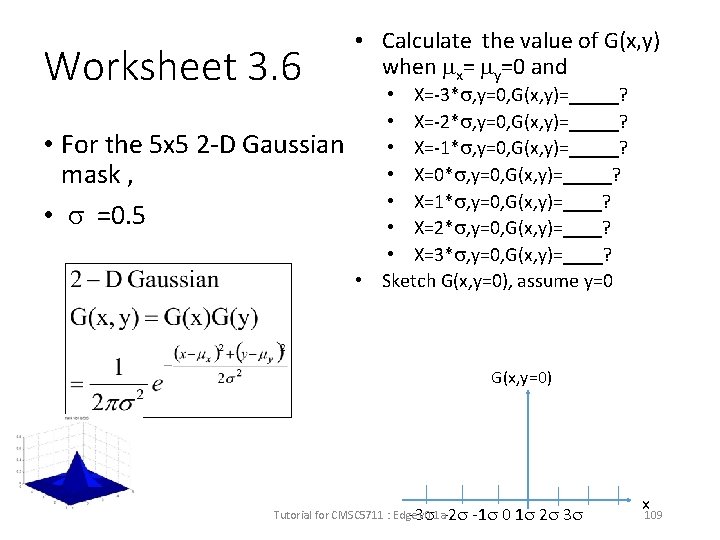
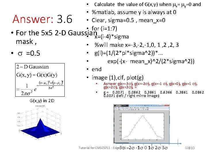
Worksheet 3. 6 • For the 5 x 5 2 -D Gaussian mask , • =0. 5 • Calculate the value of G(x, y) when x= y=0 and • X=-3* , y=0, G(x, y)=_____? • X=-2* , y=0, G(x, y)=_____? • X=-1* , y=0, G(x, y)=_____? • X=0* , y=0, G(x, y)=_____? • X=1* , y=0, G(x, y)=____? • X=2* , y=0, G(x, y)=____? • X=3* , y=0, G(x, y)=____? • Sketch G(x, y=0), assume y=0 G(x, y=0) Tutorial for CMSC 5711 : Edge v 0. 1 a-2 -3 -1 0 1 2 3 x 58

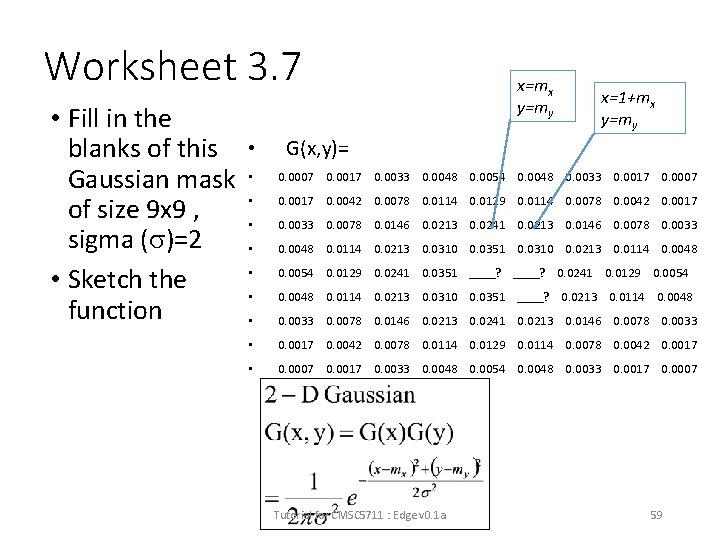
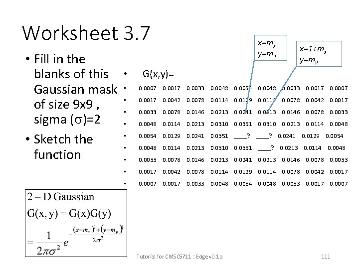
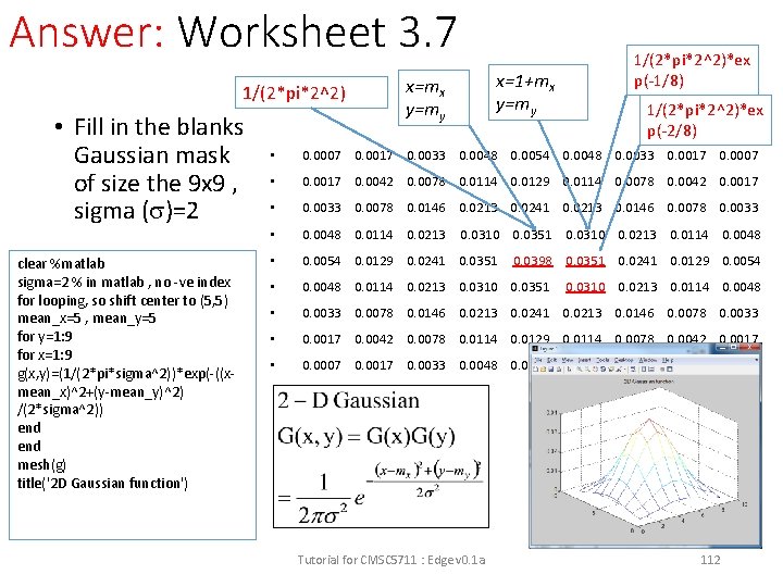
Worksheet 3. 7 • Fill in the blanks of this Gaussian mask of size 9 x 9 , sigma ( )=2 • Sketch the function • x=mx y=my x=1+mx y=my G(x, y)= • 0. 0007 0. 0017 0. 0033 0. 0048 0. 0054 0. 0048 0. 0033 0. 0017 0. 0007 • 0. 0017 0. 0042 0. 0078 0. 0114 0. 0129 0. 0114 0. 0078 0. 0042 0. 0017 • 0. 0033 0. 0078 0. 0146 0. 0213 0. 0241 0. 0213 0. 0146 0. 0078 0. 0033 • 0. 0048 0. 0114 0. 0213 0. 0310 0. 0351 0. 0310 0. 0213 0. 0114 0. 0048 • 0. 0054 0. 0129 0. 0241 0. 0351 ____? 0. 0241 0. 0129 0. 0054 • 0. 0048 0. 0114 0. 0213 0. 0310 0. 0351 ____? 0. 0213 0. 0114 0. 0048 • 0. 0033 0. 0078 0. 0146 0. 0213 0. 0241 0. 0213 0. 0146 0. 0078 0. 0033 • 0. 0017 0. 0042 0. 0078 0. 0114 0. 0129 0. 0114 0. 0078 0. 0042 0. 0017 • 0. 0007 0. 0017 0. 0033 0. 0048 0. 0054 0. 0048 0. 0033 0. 0017 0. 0007 Tutorial for CMSC 5711 : Edge v 0. 1 a 59

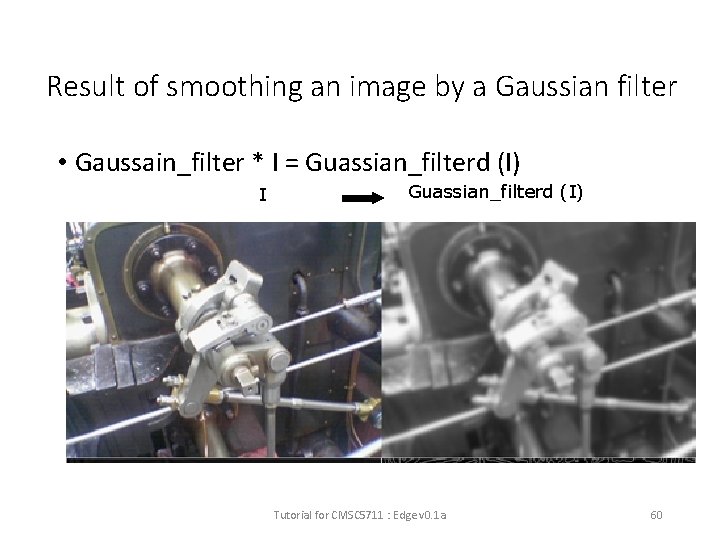
Result of smoothing an image by a Gaussian filter • Gaussain_filter * I = Guassian_filterd (I) I Guassian_filterd (I) Tutorial for CMSC 5711 : Edge v 0. 1 a 60

Laplacian filter Second order derivative method Tutorial for CMSC 5711 : Edge v 0. 1 a 61

Second order edge detection method • We use gradient G of intensity [I(x, y)] change • First order gradient • I(x, y) is an edge if I(x, y+1) I(x+1, y+1) I(x, y) I(x+1, y) I(x, y) y • Second order gradient (Laplacian operator), I(x, y) is an edge if Tutorial for CMSC 5711 : Edge v 0. 1 a x 62

Edge detection using second order gradient (Lapalcian) 2 I=G(G(I))=0 • Sharp change of intensity levels • If (intensity gradient 2 I =0) • { • pixel(x, y) is an edge point; I(x, y) • } First order derivative Second order derivative G[I(x, y)]=> threshold is an edge 2 I(x, y)= 0 is an edge Tutorial for CMSC 5711 : Edge v 0. 1 a 63

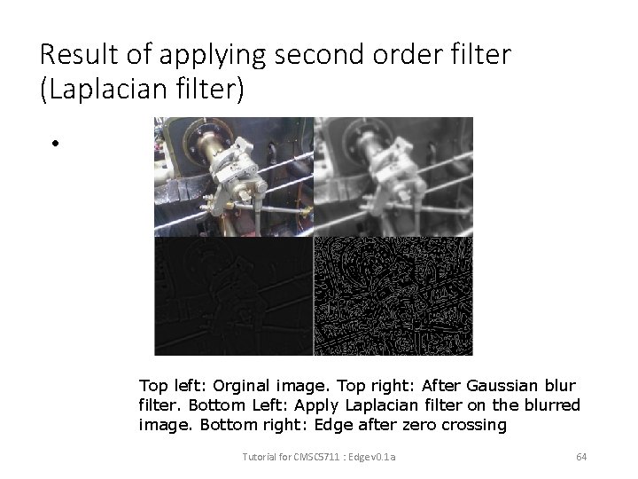
Result of applying second order filter (Laplacian filter) • Top left: Orginal image. Top right: After Gaussian blur filter. Bottom Left: Apply Laplacian filter on the blurred image. Bottom right: Edge after zero crossing Tutorial for CMSC 5711 : Edge v 0. 1 a 64

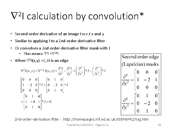
2 I calculation by convolution* • Second order derivative of an image I w. r. t x and y • Similar to applying I to a 2 nd-order-derivative filter • Or convolves a 2 nd-order-derivative filter mask with I • That means: 2 I = 2*I • When 2 I(x, y) =0, it is an edge 2 nd-order-derivative filter : http: //homepages. inf. ed. ac. uk/rbf/HIPR 2/log. htm Tutorial for CMSC 5711 : Edge v 0. 1 a 65

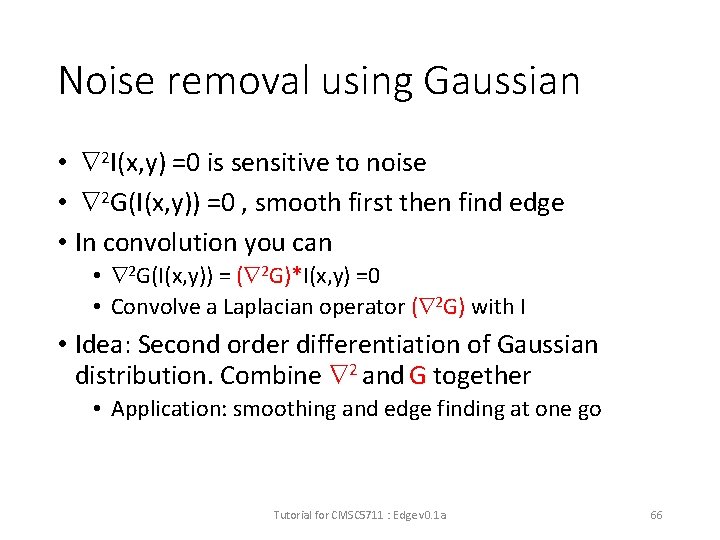
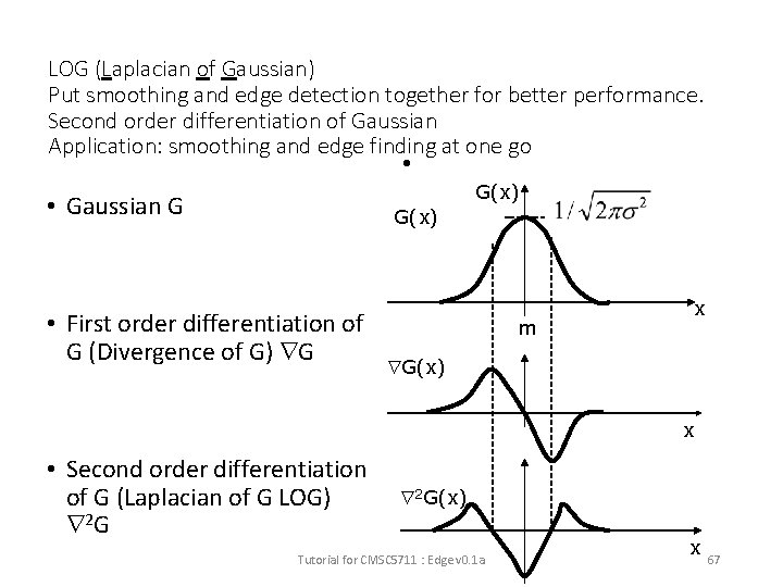
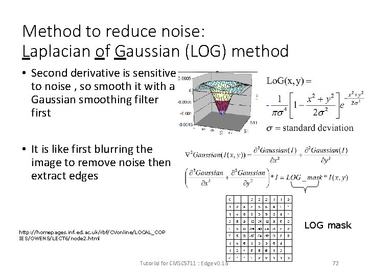
Noise removal using Gaussian • 2 I(x, y) =0 is sensitive to noise • 2 G(I(x, y)) =0 , smooth first then find edge • In convolution you can • 2 G(I(x, y)) = ( 2 G)*I(x, y) =0 • Convolve a Laplacian operator ( 2 G) with I • Idea: Second order differentiation of Gaussian distribution. Combine 2 and G together • Application: smoothing and edge finding at one go Tutorial for CMSC 5711 : Edge v 0. 1 a 66

LOG (Laplacian of Gaussian) Put smoothing and edge detection together for better performance. Second order differentiation of Gaussian Application: smoothing and edge finding at one go • G(x) • Gaussian G G(x) • First order differentiation of G (Divergence of G) G x m G(x) x • Second order differentiation of G (Laplacian of G LOG) 2 G(x) Tutorial for CMSC 5711 : Edge v 0. 1 a x 67

How to get the LOG (Laplacian of Gaussian) mask? • G(x) 1 -D Gaussian x m 2 -D Gaussian y my Tutorial for CMSC 5711 : Edge v 0. 1 a mx x 68

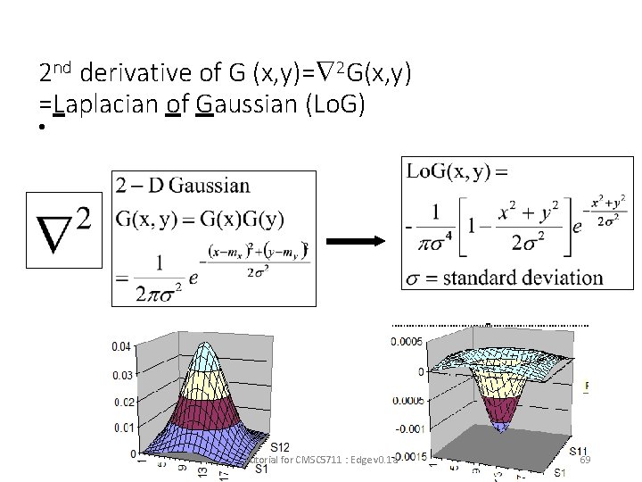
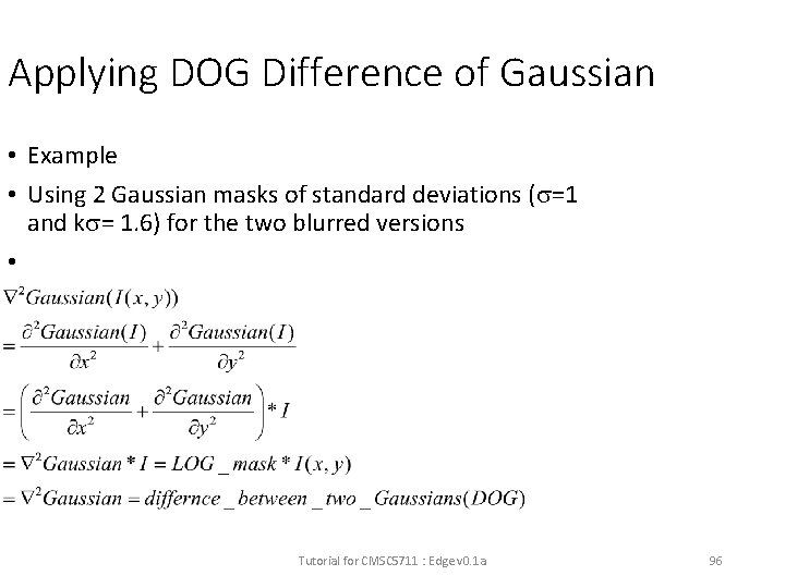
2 nd derivative of G (x, y)= 2 G(x, y) =Laplacian of Gaussian (Lo. G) • Tutorial for CMSC 5711 : Edge v 0. 1 a 69

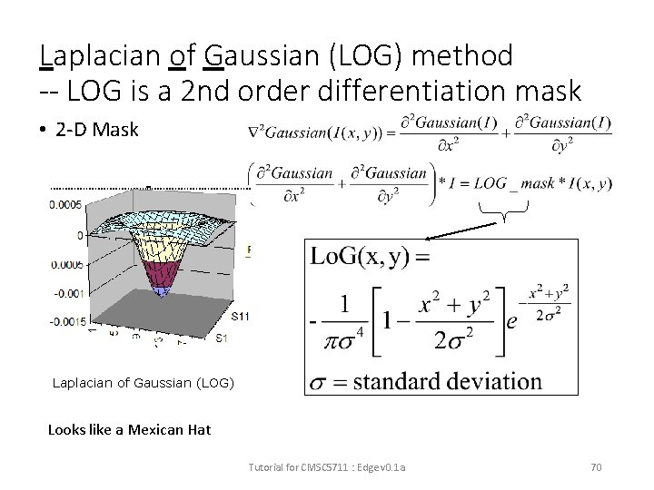
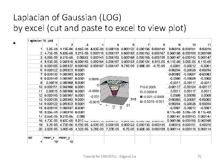
Laplacian of Gaussian (LOG) method -- LOG is a 2 nd order differentiation mask • 2 -D Mask Laplacian of Gaussian (LOG) Looks like a Mexican Hat Tutorial for CMSC 5711 : Edge v 0. 1 a 70

Laplacian of Gaussian (LOG) by excel (cut and paste to excel to view plot) • Tutorial for CMSC 5711 : Edge v 0. 1 a 71

Method to reduce noise: Laplacian of Gaussian (LOG) method • Second derivative is sensitive to noise , so smooth it with a Gaussian smoothing filter first • It is like first blurring the image to remove noise then extract edges http: //homepages. inf. ed. ac. uk/rbf/CVonline/LOCAL_COP IES/OWENS/LECT 6/node 2. html Tutorial for CMSC 5711 : Edge v 0. 1 a LOG mask 72

Canny Edge Detector p. A practical non-linear filtering method p. Very popular Tutorial for CMSC 5711 : Edge v 0. 1 a 73

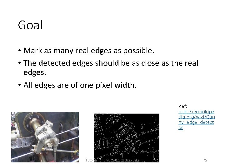
Motivation • Using 1 st derivative and 2 nd derivative alone are not good enough to locate edges • 1 st derivate method gives “thick” edges. • 2 nd derivate method gives too much noise--“rings”. • First order method with thresholding is good but too simple. It cannot handle a wide range of images. • A threshold works for one image usually won’t work for another image. Tutorial for CMSC 5711 : Edge v 0. 1 a 74

Goal • Mark as many real edges as possible. • The detected edges should be as close as the real edges. • All edges are of one pixel width. Ref: http: //en. wikipe dia. org/wiki/Can ny_edge_detect or Tutorial for CMSC 5711 : Edge v 0. 1 a 75

Canny Edge Detector • It is first proposed by John F. Canny in 1986. • Use multiple stages to detect a wide range of edges. • It uses the 1 st derivative of an image. • It takes a gray-level image as input. • Still one of the most used edge detectors in the world. Tutorial for CMSC 5711 : Edge v 0. 1 a 76

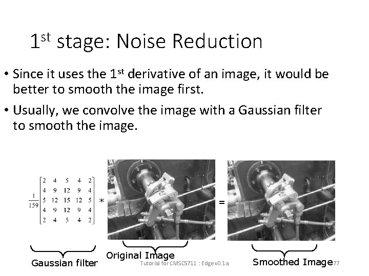
1 st stage: Noise Reduction • Since it uses the 1 st derivative of an image, it would be better to smooth the image first. • Usually, we convolve the image with a Gaussian filter to smooth the image. = * Gaussian filter Original Image Tutorial for CMSC 5711 : Edge v 0. 1 a Smoothed Image 77

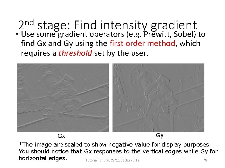
2 nd stage: Find intensity gradient • Use some gradient operators (e. g. Prewitt, Sobel) to find Gx and Gy using the first order method, which requires a threshold set by the user. Gx Gy *The image are scaled to show negative value for display purposes. You should notice that Gx responses to the vertical edges while Gy for horizontal edges. Tutorial for CMSC 5711 : Edge v 0. 1 a 78

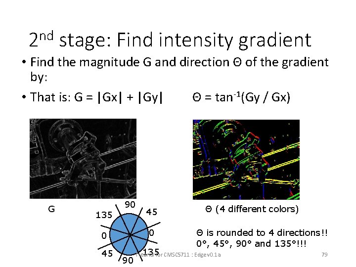
2 nd stage: Find intensity gradient • Find the magnitude G and direction Θ of the gradient by: • That is: G = |Gx| + |Gy| Θ = tan-1(Gy / Gx) G 135 90 0 0 45 45 90 Θ (4 different colors) Θ is rounded to 4 directions!! 0°, 45°, 90° and 135°!!! 135 for CMSC 5711 : Edge v 0. 1 a Tutorial 79

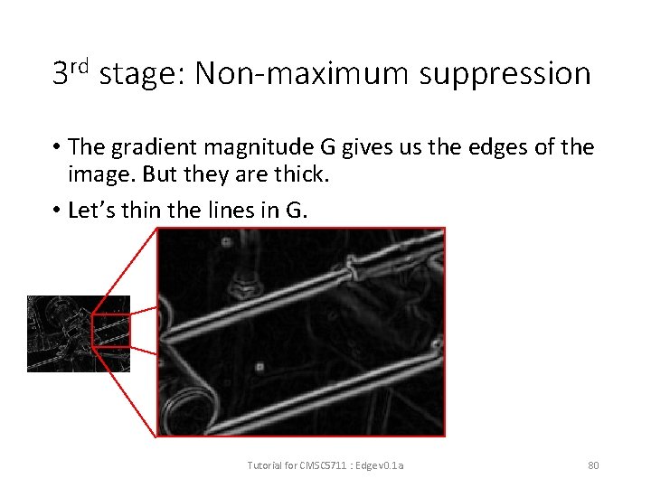
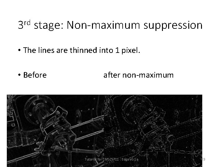
3 rd stage: Non-maximum suppression • The gradient magnitude G gives us the edges of the image. But they are thick. • Let’s thin the lines in G. Tutorial for CMSC 5711 : Edge v 0. 1 a 80

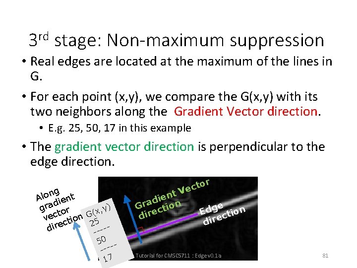
3 rd stage: Non-maximum suppression • Real edges are located at the maximum of the lines in G. • For each point (x, y), we compare the G(x, y) with its two neighbors along the Gradient Vector direction. • E. g. 25, 50, 17 in this example • The gradient vector direction is perpendicular to the edge direction. ng Alo ient d gra or , y) x ( t vec ction G 5 2 dire ---- 50 ---17 or t Vec ent i d Gra ction e dir e Edg ction e dir Tutorial for CMSC 5711 : Edge v 0. 1 a 81

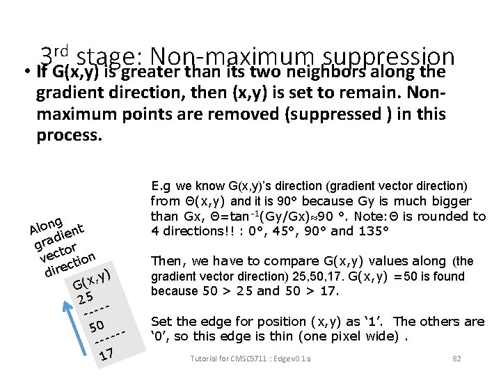
rd stage: Non-maximum suppression 3 • If G(x, y) is greater than its two neighbors along the gradient direction, then (x, y) is set to remain. Nonmaximum points are removed (suppressed ) in this process. ng Alo ient d gra or t vec ction dire , y) x ( G 25 ---50 ----17 E. g we know G(x, y)’s direction (gradient vector direction) from Θ(x, y) and it is 90° because Gy is much bigger than Gx, Θ=tan-1(Gy/Gx) 90 °. Note: Θ is rounded to 4 directions!! : 0°, 45°, 90° and 135° Then, we have to compare G(x, y) values along (the gradient vector direction) 25, 50, 17. G(x, y) =50 is found because 50 > 25 and 50 > 17. Set the edge for position (x, y) as ‘ 1’. The others are ‘ 0’, so this edge is thin (one pixel wide). Tutorial for CMSC 5711 : Edge v 0. 1 a 82

3 rd stage: Non-maximum suppression • The lines are thinned into 1 pixel. • Before after non-maximum Tutorial for CMSC 5711 : Edge v 0. 1 a 83

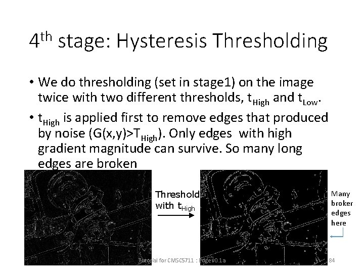
4 th stage: Hysteresis Thresholding • We do thresholding (set in stage 1) on the image twice with two different thresholds, t. High and t. Low. • t. High is applied first to remove edges that produced by noise (G(x, y)>THigh). Only edges with high gradient magnitude can survive. So many long edges are broken Threshold with t. High Tutorial for CMSC 5711 : Edge v 0. 1 a Many broker edges here 84

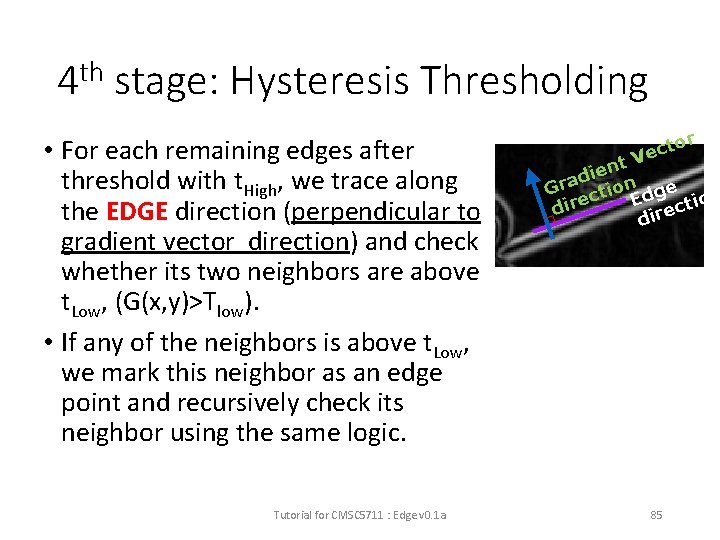
4 th stage: Hysteresis Thresholding • For each remaining edges after threshold with t. High, we trace along the EDGE direction (perpendicular to gradient vector direction) and check whether its two neighbors are above t. Low, (G(x, y)>Tlow). • If any of the neighbors is above t. Low, we mark this neighbor as an edge point and recursively check its neighbor using the same logic. Tutorial for CMSC 5711 : Edge v 0. 1 a r to c e V ent i d Gra ction dge e E ion t c dir e dir 85

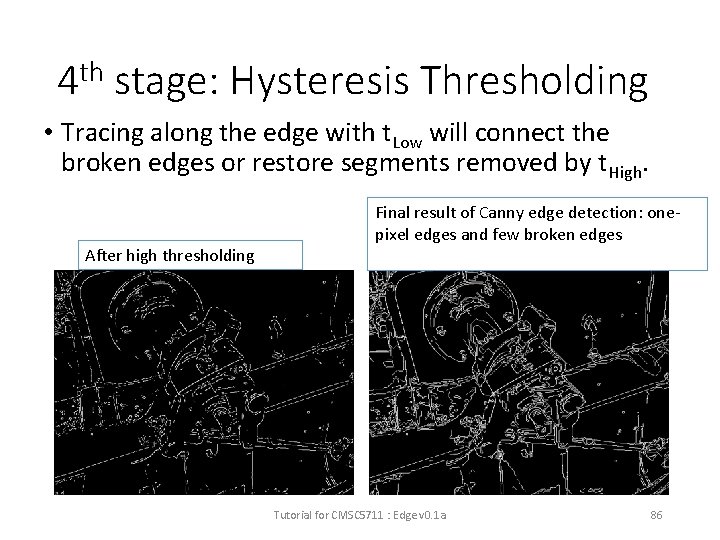
4 th stage: Hysteresis Thresholding • Tracing along the edge with t. Low will connect the broken edges or restore segments removed by t. High. After high thresholding Final result of Canny edge detection: onepixel edges and few broken edges Tutorial for CMSC 5711 : Edge v 0. 1 a 86

Open. CV • Since Canny edge detector is so popular, Intel’s Computer Vision library, namely Open. CV, has included this detector. • You can just call the build-in function Canny() and put corresponding parameters (e. g. the two thresholds) in it. • It is highly optimized and can be run in real time with a normal PC and Webcam. • More information: http: //opencv. willowgarage. com/documentation/cpp/feature_detectio n. html? highlight=canny#Canny • http: //www. pages. drexel. edu/~weg 22/can_tut. html Tutorial for CMSC 5711 : Edge v 0. 1 a 87

Writing your own Canny edge detector • If you want to implement it yourself, you can still use Open. CV since it provides a lot of useful functions like Sobel() and gaussian. Blur(). Tutorial for CMSC 5711 : Edge v 0. 1 a 88

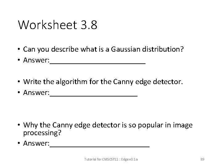
Worksheet 3. 8 • Can you describe what is a Gaussian distribution? • Answer: ____________ • Write the algorithm for the Canny edge detector. • Answer: ___________ • Why the Canny edge detector is so popular in image processing? • Answer: _____________ Tutorial for CMSC 5711 : Edge v 0. 1 a 89

Conclusion • Studied first order and second order edge detection techniques • Studied the Gaussian operator • Studied the Canny edge detection algorithm Tutorial for CMSC 5711 : Edge v 0. 1 a 90

Appendix Tutorial for CMSC 5711 : Edge v 0. 1 a 91

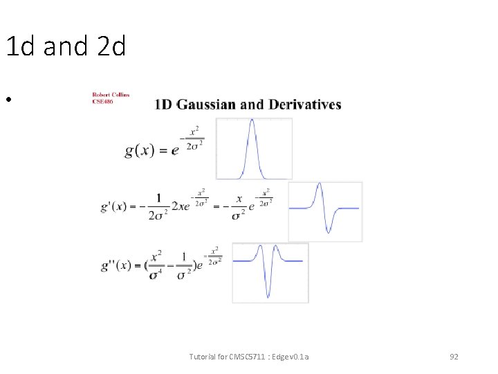
1 d and 2 d • Tutorial for CMSC 5711 : Edge v 0. 1 a 92

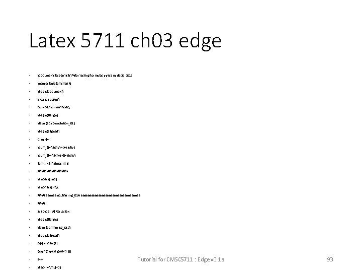
Latex 5711 ch 03 edge • documentclass{article} %for testing formulas ppt cam, dec 8, 2019 • usepackage{amsmath} • begin{document} • 5711 03 edge\ • Convolution method\ • begin{flalign} • label{eq: convolution_01} • begin{aligned} • C(m, n)= • sum_{j=-infty}^{j=infty} • sum_{k=-infty}^{j=infty} • h(m-j, n-k) times I(j, k) • %%%%%% • end{aligned} • end{flalign}\ • %%% eeeeee eq: filtering_01 A eeeeeeeeeeeeeeeee • %%% • 1 st order (A) Gaussian • begin{flalign} • label{eq: filtering_01 a} • begin{aligned} • G(x) = frac{1} • {sqrt{2pi{sigma^2 }}} • e^{- • frac{(x-mu)^2} Tutorial for CMSC 5711 : Edge v 0. 1 a 93

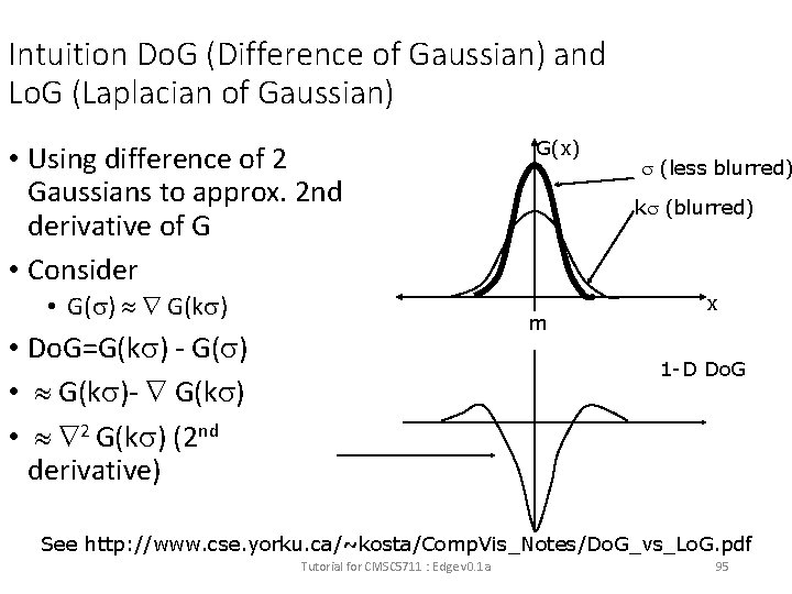
Obtain a LOG mask by Do. F Difference of Gaussian • Want to remove noise with low frequency (low fluctuation) and high frequency (high fluctuation). • That means band pass filtering • Solution • Difference of Gaussians Do. G= • (Blurred version of I) – (Less blurred version of I) • Do. G=G(k )- G( ) Tutorial for CMSC 5711 : Edge v 0. 1 a 94

Intuition Do. G (Difference of Gaussian) and Lo. G (Laplacian of Gaussian) • Using difference of 2 Gaussians to approx. 2 nd derivative of G • Consider • G( ) G(k ) G(x) k (blurred) m • Do. G=G(k ) - G( ) • G(k )- G(k ) • 2 G(k ) (2 nd derivative) (less blurred) x 1 -D Do. G See http: //www. cse. yorku. ca/~kosta/Comp. Vis_Notes/Do. G_vs_Lo. G. pdf Tutorial for CMSC 5711 : Edge v 0. 1 a 95

Applying DOG Difference of Gaussian • Example • Using 2 Gaussian masks of standard deviations ( =1 and k = 1. 6) for the two blurred versions • Tutorial for CMSC 5711 : Edge v 0. 1 a 96

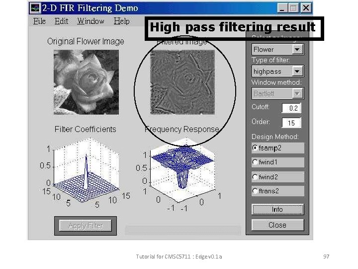
High pass filtering result Tutorial for CMSC 5711 : Edge v 0. 1 a 97

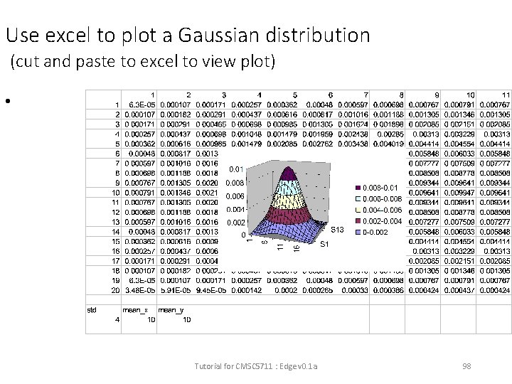
Use excel to plot a Gaussian distribution (cut and paste to excel to view plot) • Tutorial for CMSC 5711 : Edge v 0. 1 a 98

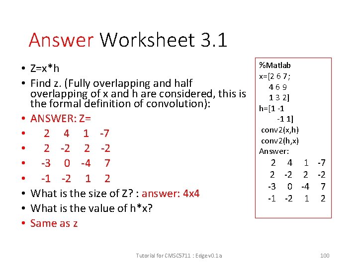
Cmsc 5711, Worksheet 3. 1 x=[2 6 7; 469 1 3 2] h=[1 -1 -1 1] Z=x*h % * is the convolution operator Find z. (Fully overlapping and half overlapping of x and h are considered, this is the formal definition of convolution) • What is the size of Z? • What is the value of h*x? • • Tutorial for CMSC 5711 : Edge v 0. 1 a 99

Answer Worksheet 3. 1 • Z=x*h • Find z. (Fully overlapping and half overlapping of x and h are considered, this is the formal definition of convolution): • ANSWER: Z= • 2 4 1 -7 • 2 -2 • -3 0 -4 7 • -1 -2 1 2 • What is the size of Z? : answer: 4 x 4 • What is the value of h*x? • Same as z Tutorial for CMSC 5711 : Edge v 0. 1 a %Matlab x=[2 6 7; 469 1 3 2] h=[1 -1 -1 1] conv 2(x, h) conv 2(h, x) Answer: 2 4 1 -7 2 -2 -3 0 -4 7 -1 -2 1 2 100

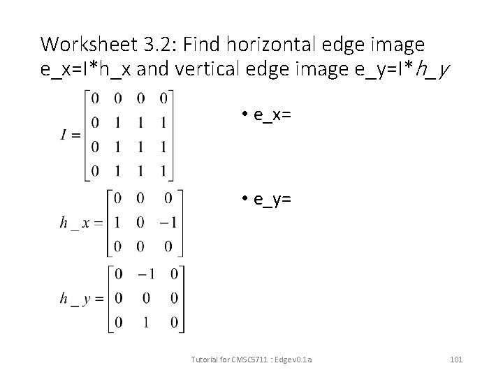
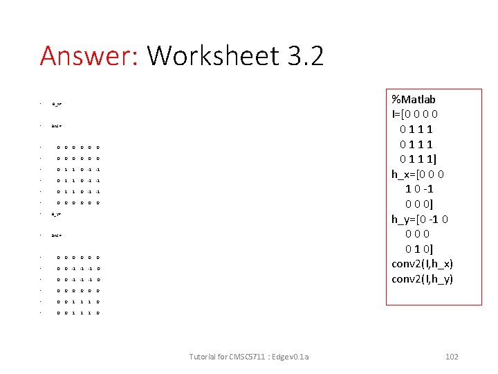
Worksheet 3. 2: Find horizontal edge image e_x=I*h_x and vertical edge image e_y=I*h_y • e_x= • e_y= Tutorial for CMSC 5711 : Edge v 0. 1 a 101

Answer: Worksheet 3. 2 • e_x= • ans = • 0 0 0 • 0 1 1 0 -1 -1 • 0 0 0 0 • e_y= • ans = • 0 0 -1 -1 -1 0 • 0 0 1 1 1 0 %Matlab I=[0 0 0111 0 1 1 1] h_x=[0 0 0 1 0 -1 0 0 0] h_y=[0 -1 0 000 0 1 0] conv 2(I, h_x) conv 2(I, h_y) Tutorial for CMSC 5711 : Edge v 0. 1 a 102

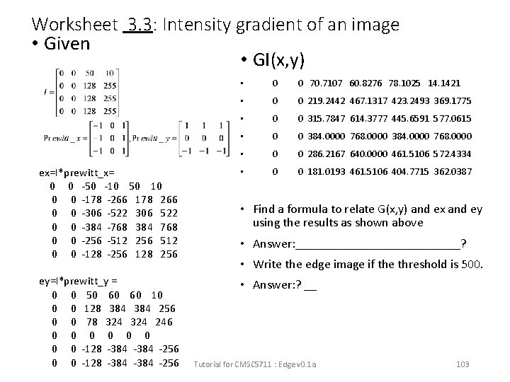
Worksheet 3. 3: Intensity gradient of an image • Given • GI(x, y) • 0 0 70. 7107 60. 8276 78. 1025 14. 1421 • 0 0 219. 2442 467. 1317 423. 2493 369. 1775 • 0 0 315. 7847 614. 3777 445. 6591 577. 0615 • 0 0 384. 0000 768. 0000 • 0 0 286. 2167 640. 0000 461. 5106 572. 4334 ex=I*prewitt_x= 0 0 -50 -10 50 10 0 0 -178 -266 178 266 0 0 -306 -522 306 522 0 0 -384 -768 384 768 0 0 -256 -512 256 512 0 0 -128 -256 128 256 • 0 0 181. 0193 461. 5106 404. 7715 362. 0387 ey=I*prewitt_y = 0 0 50 60 60 10 0 0 128 384 256 0 0 78 324 246 0 0 0 0 -128 -384 -256 • Answer: ? __ • Find a formula to relate G(x, y) and ex and ey using the results as shown above • Answer: _____________? • Write the edge image if the threshold is 500. Tutorial for CMSC 5711 : Edge v 0. 1 a 103

Answer: Worksheet 3. 3: Intensity gradient of an image %Answer: matlab I=[ 0 0 50 10 0 0 128 256] pr_x=[-1 0 1] pr_y=[1 1 1 0 00 -1 -1 -1] e_x=conv 2(I, pr_x) e_y=conv 2(I, pr_y) e_total=sqrt(e_x. ^2+e_y. ^2) ex=I*prewitt_x= 0 0 -50 -10 50 10 0 0 -178 -266 178 266 0 0 -306 -522 306 522 0 0 -384 -768 384 768 0 0 -256 -512 256 512 0 0 -128 -256 128 256 ey=I*prewitt_y = 0 0 50 60 60 10 0 0 128 384 256 0 0 78 324 246 0 0 0 0 -128 -384 -256 • GI(x, y) • 0 0 70. 7107 60. 8276 78. 1025 14. 1421 • 0 0 219. 2442 467. 1317 423. 2493 369. 1775 • 0 0 315. 7847 614. 3777 445. 6591 577. 0615 • 0 0 384. 0000 768. 0000 • 0 0 286. 2167 640. 0000 461. 5106 572. 4334 • 0 0 181. 0193 461. 5106 404. 7715 362. 0387 • Find a formula to relate G(x, y) and ex and ey • using the results as shown above • Answer: GI(x, y)=sqrt{ ex(x, y)^2 + ey(x, y)^2 } • Write the edge image if the threshold is 500. Or G(x, y)= • 0 0 070. 7107 060. 8276 078. 1025 014. 1421 • 0 0 0219. 2442 0467. 1317 0423. 2493 0369. 1775 • 0 0 0315. 7847 1614. 3777 0445. 6591 1577. 0615 • 0 0 0384. 0000 1768. 0000 • 0 0 0286. 2167 1640. 0000 0461. 5106 1572. 4334 • 0 0 0181. 0193 0461. 5106 0404. 7715 0362. 0387 • Or edge(x, y) • 000000 • 000101 • 000000 Tutorial for CMSC 5711 : Edge v 0. 1 a If G(x, y) >500, edge(x, y)=1 else edge(x, y)=0 • 104

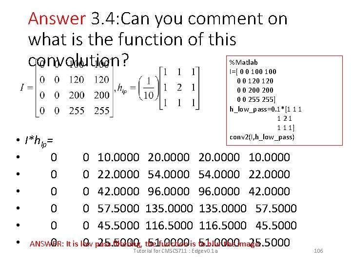
Worksheet 3. 4: Can you comment on what is the function of this convolution? • I*hlp= • 0 • 0 • 0 0 0 0 10. 0000 22. 0000 42. 0000 57. 5000 45. 5000 20. 0000 54. 0000 96. 0000 135. 0000 116. 5000 51. 0000 20. 0000 10. 0000 54. 0000 22. 0000 96. 0000 42. 0000 135. 0000 57. 5000 116. 5000 45. 5000 51. 0000 25. 5000 Tutorial for CMSC 5711 : Edge v 0. 1 a 105

Answer 3. 4: Can you comment on what is the function of this convolution? %Matlab I=[ 0 0 100 0 0 120 0 0 200 0 0 255] h_low_pass=0. 1*[1 1 1 121 1 1 1] conv 2(I, h_low_pass) • I*hlp= • 0 0 10. 0000 20. 0000 10. 0000 • 0 0 22. 0000 54. 0000 22. 0000 • 0 0 42. 0000 96. 0000 42. 0000 • 0 0 57. 5000 135. 0000 57. 5000 • 0 0 45. 5000 116. 5000 45. 5000 • ANSWER: 0 It is low 0 pass 25. 5000 51. 0000 25. 5000 filtering, the function is to blur the image. Tutorial for CMSC 5711 : Edge v 0. 1 a 106

Worksheet 3. 5: Example for intensity gradient calculation • Given ex=I*prewitt_x= 0 0 -50 -10 50 10 0 0 -178 -266 178 266 0 0 -306 -522 306 522 0 0 -384 -768 384 768 0 0 -256 -512 256 512 0 0 -128 -256 128 256 ey=I*prewitt_y = 0 0 50 60 60 10 0 0 128 384 256 0 0 78 324 246 0 0 0 0 -128 -384 -256 • GI(x, y) (x 1, y 1) • 0 0 70. 7107 60. 8276 78. 1025 14. 1421 • 0 0 219. 2442 467. 1317 423. 2493 369. 1775 • 0 0 315. 7847 614. 3777 445. 6591 577. 0615 • 0 0 384. 0000 768. 0000 • 0 0 286. 2167 640. 0000 461. 5106 572. 4334 • 0 0 181. 0193 461. 5106 404. 7715 362. 0387 • Write a formula to find the direction of the edge image at pixel (x, y). • Answer: ________? • Find the edge direction at (x 1, y 1) • Answer: ________? Tutorial for CMSC 5711 : Edge v 0. 1 a 107

Answer: Worksheet 3. 5: Example for intensity gradient calculation • Given ex=I*prewitt_x= 0 0 -50 -10 50 10 0 0 -178 -266 178 266 0 0 -306 -522 306 522 0 0 -384 -768 384 768 0 0 -256 -512 256 512 0 0 -128 -256 128 256 ey=I*prewitt_y = 0 0 50 60 60 10 0 0 128 384 256 0 0 78 324 246 0 0 0 0 -128 -384 -256 • GI(x, y) (x 1, y 1) • 0 0 70. 7107 60. 8276 78. 1025 14. 1421 • 0 0 219. 2442 467. 1317 423. 2493 369. 1775 • 0 0 315. 7847 614. 3777 445. 6591 577. 0615 • 0 0 384. 0000 768. 0000 • 0 0 286. 2167 640. 0000 461. 5106 572. 4334 • 0 0 181. 0193 461. 5106 404. 7715 362. 0387 • Write a formula to find the direction of the edge image at pixel (x, y) • Answer: Θ(x, y) = tan-1(ey(x, y) / ex(x, y)) • Find the edge direction at (x 1, y 1) • Answer: Θ(x 1, y 1) = tan-1(ey(x 1, y 1) / ex(x 1, y 1)) • Θ(x, y) =atan(384/(-266)) • =-0. 964980881 rad Tutorial for CMSC 5711 : Edge v 0. 1 a 108

Worksheet 3. 6 • For the 5 x 5 2 -D Gaussian mask , • =0. 5 • Calculate the value of G(x, y) when x= y=0 and • X=-3* , y=0, G(x, y)=_____? • X=-2* , y=0, G(x, y)=_____? • X=-1* , y=0, G(x, y)=_____? • X=0* , y=0, G(x, y)=_____? • X=1* , y=0, G(x, y)=____? • X=2* , y=0, G(x, y)=____? • X=3* , y=0, G(x, y)=____? • Sketch G(x, y=0), assume y=0 G(x, y=0) Tutorial for CMSC 5711 : Edge v 0. 1 a-2 -3 -1 0 1 2 3 x 109

• Calculate the value of G(x, y) when x= y=0 and • %matlab, assume y is always at 0 • Clear, sigma=0. 5 , mean_x=0 • for (i=1: 7) For the 5 x 5 2 -D Gaussian • x=(i-4)*sigma mask , • %will make x=-3, -2, -1, 0, 1 , 2, 3 • g(i)=(1/(2*pi*sigma^2))*. . . =0. 5 • exp(-(x- mean_x)^2/(2*sigma^2)) • end • image (1), clf, plot(g) Answer: 3. 6 • • G(x, y) in 2 D Asnwer g(x=-3 ), g(x=-2 ), g(x=-1 ), g(x=0), g(x=1 ), g(x=2 ), g(x=3 ), = g = 0. 0071 0. 0862 0. 3861 0. 6366 0. 3861 0. 0862 0. 0071 (left / right mirro image) Tutorial for CMSC 5711 : Edge v 0. 1 a-2 -3 -1 0 1 2 3 110

Worksheet 3. 7 • Fill in the blanks of this Gaussian mask of size 9 x 9 , sigma ( )=2 • Sketch the function • x=mx y=my x=1+mx y=my G(x, y)= • 0. 0007 0. 0017 0. 0033 0. 0048 0. 0054 0. 0048 0. 0033 0. 0017 0. 0007 • 0. 0017 0. 0042 0. 0078 0. 0114 0. 0129 0. 0114 0. 0078 0. 0042 0. 0017 • 0. 0033 0. 0078 0. 0146 0. 0213 0. 0241 0. 0213 0. 0146 0. 0078 0. 0033 • 0. 0048 0. 0114 0. 0213 0. 0310 0. 0351 0. 0310 0. 0213 0. 0114 0. 0048 • 0. 0054 0. 0129 0. 0241 0. 0351 ____? 0. 0241 0. 0129 0. 0054 • 0. 0048 0. 0114 0. 0213 0. 0310 0. 0351 ____? 0. 0213 0. 0114 0. 0048 • 0. 0033 0. 0078 0. 0146 0. 0213 0. 0241 0. 0213 0. 0146 0. 0078 0. 0033 • 0. 0017 0. 0042 0. 0078 0. 0114 0. 0129 0. 0114 0. 0078 0. 0042 0. 0017 • 0. 0007 0. 0017 0. 0033 0. 0048 0. 0054 0. 0048 0. 0033 0. 0017 0. 0007 Tutorial for CMSC 5711 : Edge v 0. 1 a 111

Answer: Worksheet 3. 7 1/(2*pi*2^2) • Fill in the blanks Gaussian mask of size the 9 x 9 , sigma ( )=2 clear %matlab sigma=2 % in matlab , no -ve index for looping, so shift center to (5, 5) mean_x=5 , mean_y=5 for y=1: 9 for x=1: 9 g(x, y)=(1/(2*pi*sigma^2))*exp(-((xmean_x)^2+(y-mean_y)^2) /(2*sigma^2)) end mesh(g) title('2 D Gaussian function') x=1+mx y=my x=mx y=my 1/(2*pi*2^2)*ex p(-1/8) 1/(2*pi*2^2)*ex p(-2/8) • 0. 0007 0. 0017 0. 0033 0. 0048 0. 0054 0. 0048 0. 0033 0. 0017 0. 0007 • 0. 0017 0. 0042 0. 0078 0. 0114 0. 0129 0. 0114 0. 0078 0. 0042 0. 0017 • 0. 0033 0. 0078 0. 0146 0. 0213 0. 0241 0. 0213 0. 0146 0. 0078 0. 0033 • 0. 0048 0. 0114 0. 0213 • 0. 0054 0. 0129 0. 0241 0. 0351 • 0. 0048 0. 0114 0. 0213 0. 0310 0. 0351 • 0. 0033 0. 0078 0. 0146 0. 0213 0. 0241 0. 0213 0. 0146 0. 0078 0. 0033 • 0. 0017 0. 0042 0. 0078 0. 0114 0. 0129 0. 0114 0. 0078 0. 0042 0. 0017 • 0. 0007 0. 0017 0. 0033 0. 0048 0. 0054 0. 0048 0. 0033 0. 0017 0. 0007 0. 0310 0. 0351 0. 0310 0. 0213 0. 0114 0. 0048 Tutorial for CMSC 5711 : Edge v 0. 1 a 0. 0398 0. 0351 0. 0241 0. 0129 0. 0054 0. 0310 0. 0213 0. 0114 0. 0048 112

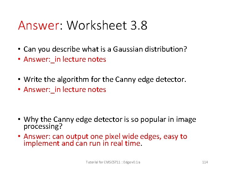
Worksheet 3. 8 • Can you describe what is a Gaussian distribution? • Answer: ____________ • Write the algorithm for the Canny edge detector. • Answer: ___________ • Why the Canny edge detector is so popular in image processing? • Answer: _____________ Tutorial for CMSC 5711 : Edge v 0. 1 a 113

Answer: Worksheet 3. 8 • Can you describe what is a Gaussian distribution? • Answer: _in lecture notes • Write the algorithm for the Canny edge detector. • Answer: _in lecture notes • Why the Canny edge detector is so popular in image processing? • Answer: can output one pixel wide edges, easy to implement and can run in real time. Tutorial for CMSC 5711 : Edge v 0. 1 a 114