CCD Image Processing Issues Solutions Correction of Raw

CCD Image Processing: Issues & Solutions

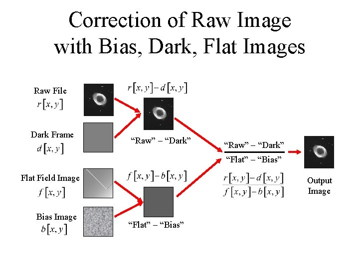
Correction of Raw Image with Bias, Dark, Flat Images Raw File Dark Frame “Raw” “Dark” “Flat” “Bias” Flat Field Image Bias Image Output Image “Flat” “Bias”

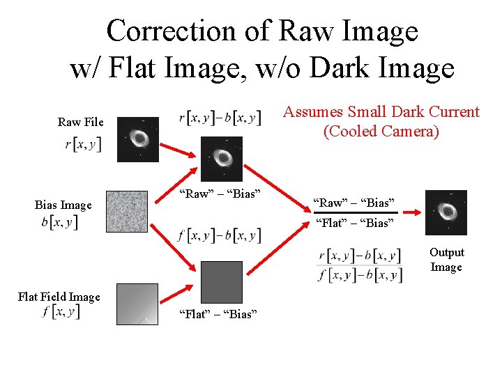
Correction of Raw Image w/ Flat Image, w/o Dark Image Assumes Small Dark Current (Cooled Camera) Raw File Bias Image “Raw” “Bias” “Flat” “Bias” Output Image Flat Field Image “Flat” “Bias”

CCDs: Noise Sources • Sky “Background” – Diffuse Light from Sky (Usually Variable) • Dark Current – Signal from Unexposed CCD – Due to Electronic Amplifiers • Photon Counting – Uncertainty in Number of Incoming Photons • Read Noise – Uncertainty in Number of Electrons at a Pixel

Problem with Sky “Background” • Uncertainty in Number of Photons from Source – “How much signal is actually from the source object instead of intervening atmosphere?

Solution for Sky Background • Measure Sky Signal from Images – Taken in (Approximately) Same Direction (Region of Sky) at (Approximately) Same Time – Use “Off-Object” Region(s) of Source Image • Subtract Brightness Values from Object Values

Problem: Dark Current • Signal in Every Pixel Even if NOT Exposed to Light – Strength Proportional to Exposure Time • Signal Varies Over Pixels – Non-Deterministic Signal = “NOISE”

Solution: Dark Current • Subtract Image(s) Obtained Without Exposing CCD – Leave Shutter Closed to Make a “Dark Frame” – Same Exposure Time for Image and Dark Frame • Measure of “Similar” Noise as in Exposed Image • Actually Average Measurements from Multiple Images – Decreases “Uncertainty” in Dark Current

Digression on “Noise” • What is “Noise”? • Noise is a “Nondeterministic” Signal – “Random” Signal – Exact Form is not Predictable – “Statistical” Properties ARE (usually) Predictable

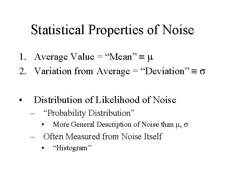
Statistical Properties of Noise 1. Average Value = “Mean” 2. Variation from Average = “Deviation” • Distribution of Likelihood of Noise – “Probability Distribution” • More General Description of Noise than , – Often Measured from Noise Itself • “Histogram”

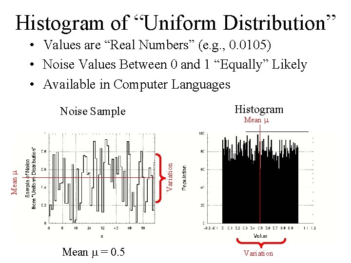
Histogram of “Uniform Distribution” • Values are “Real Numbers” (e. g. , 0. 0105) • Noise Values Between 0 and 1 “Equally” Likely • Available in Computer Languages Histogram Noise Sample Mean Variation Mean = 0. 5 Variation

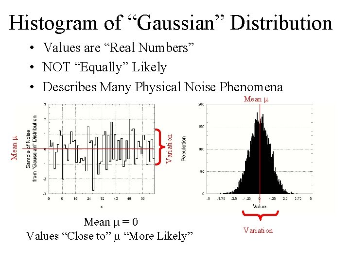
Histogram of “Gaussian” Distribution • Values are “Real Numbers” • NOT “Equally” Likely • Describes Many Physical Noise Phenomena Variation Mean = 0 Values “Close to” “More Likely” Variation

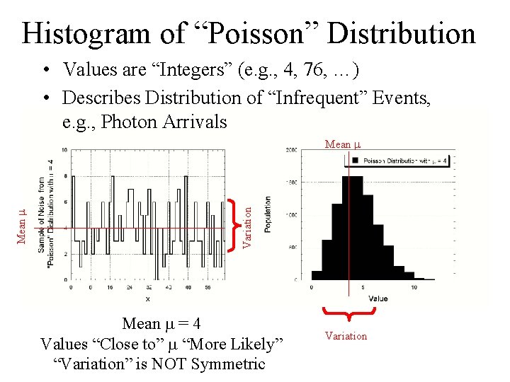
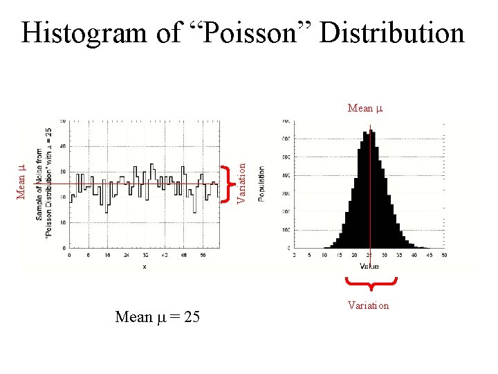
Histogram of “Poisson” Distribution • Values are “Integers” (e. g. , 4, 76, …) • Describes Distribution of “Infrequent” Events, e. g. , Photon Arrivals Variation Mean = 4 Values “Close to” “More Likely” “Variation” is NOT Symmetric Variation

Histogram of “Poisson” Distribution Mean Variation Mean = 25 Variation

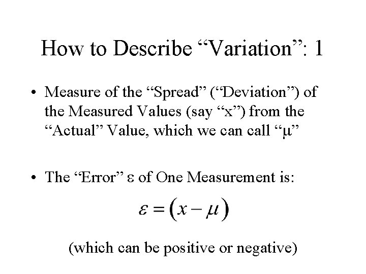
How to Describe “Variation”: 1 • Measure of the “Spread” (“Deviation”) of the Measured Values (say “x”) from the “Actual” Value, which we can call “ ” • The “Error” of One Measurement is: (which can be positive or negative)

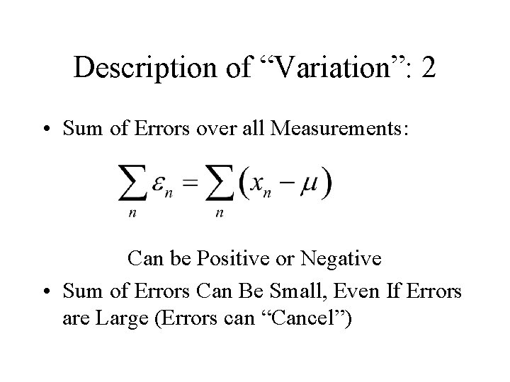
Description of “Variation”: 2 • Sum of Errors over all Measurements: Can be Positive or Negative • Sum of Errors Can Be Small, Even If Errors are Large (Errors can “Cancel”)

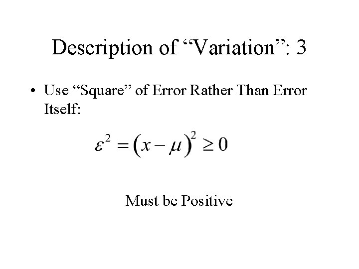
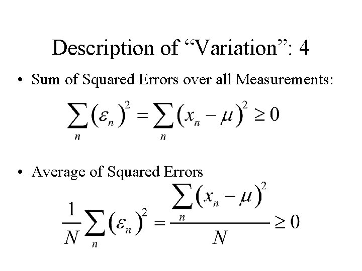
Description of “Variation”: 3 • Use “Square” of Error Rather Than Error Itself: Must be Positive

Description of “Variation”: 4 • Sum of Squared Errors over all Measurements: • Average of Squared Errors

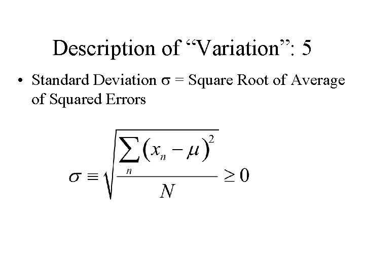
Description of “Variation”: 5 • Standard Deviation = Square Root of Average of Squared Errors

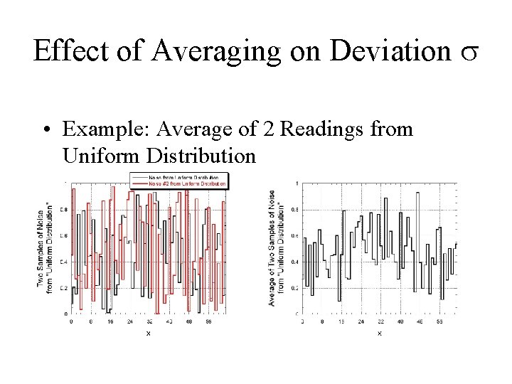
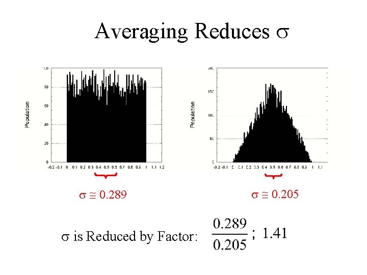
Effect of Averaging on Deviation • Example: Average of 2 Readings from Uniform Distribution

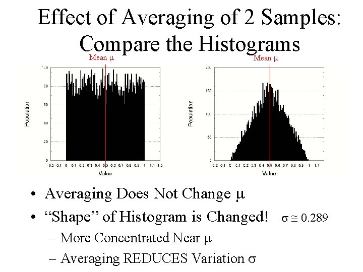
Effect of Averaging of 2 Samples: Compare the Histograms Mean • Averaging Does Not Change • “Shape” of Histogram is Changed! – More Concentrated Near – Averaging REDUCES Variation 0. 289

Averaging Reduces 0. 289 is Reduced by Factor: 0. 205

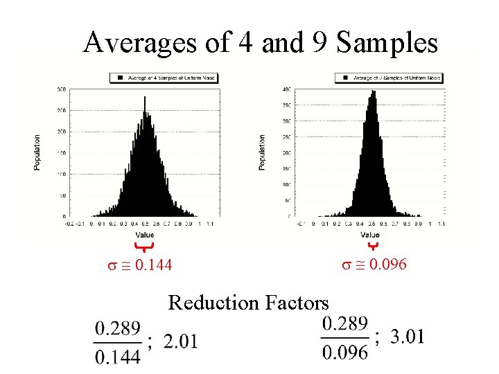
Averages of 4 and 9 Samples 0. 144 Reduction Factors 0. 096

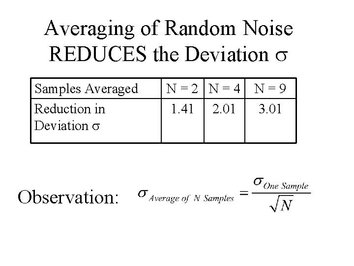
Averaging of Random Noise REDUCES the Deviation Samples Averaged Reduction in Deviation Observation: N=2 N=4 1. 41 2. 01 N=9 3. 01

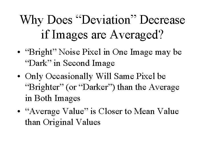
Why Does “Deviation” Decrease if Images are Averaged? • “Bright” Noise Pixel in One Image may be “Dark” in Second Image • Only Occasionally Will Same Pixel be “Brighter” (or “Darker”) than the Average in Both Images • “Average Value” is Closer to Mean Value than Original Values

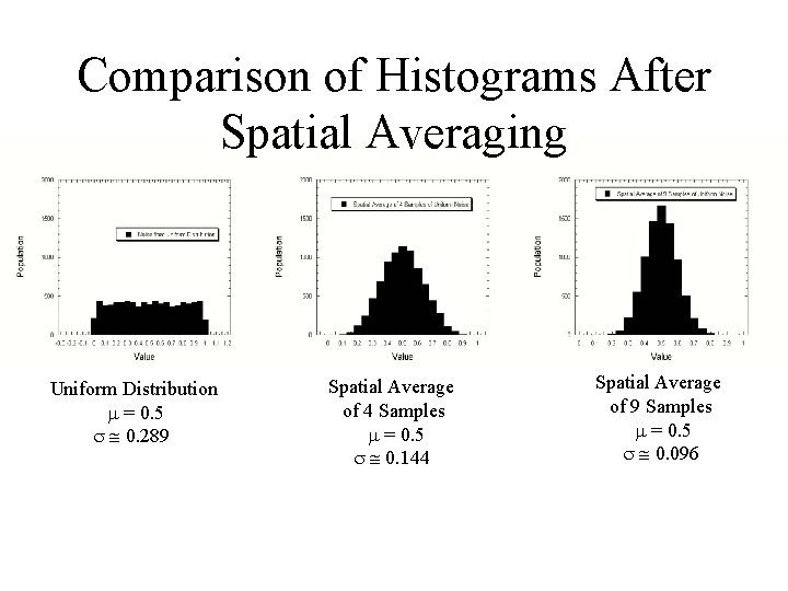
Averaging Over “Time” vs. Averaging Over “Space” • Examples of Averaging Different Noise Samples Collected at Different Times • Could Also Average Different Noise Samples Over “Space” (i. e. , Coordinate x) – “Spatial Averaging”

Comparison of Histograms After Spatial Averaging Uniform Distribution = 0. 5 0. 289 Spatial Average of 4 Samples = 0. 5 0. 144 Spatial Average of 9 Samples = 0. 5 0. 096

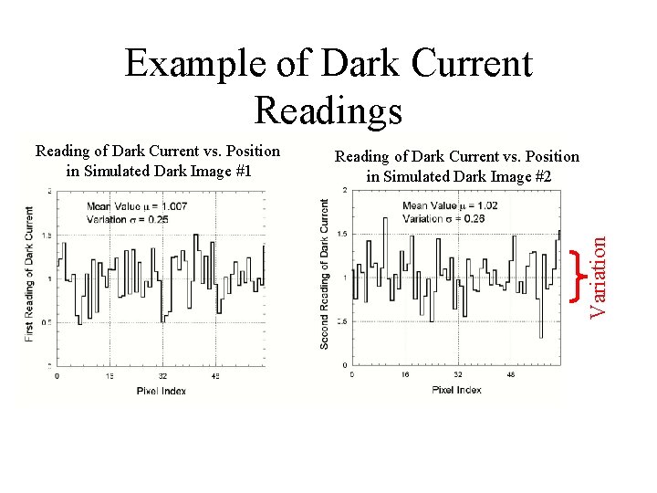
Effect of Averaging on Dark Current • Dark Current is NOT a “Deterministic” Number – Each Measurement of Dark Current “Should Be” Different – Values Are Selected from Some Distribution of Likelihood (Probability)

Example of Dark Current • One-Dimensional Examples (1 -D Functions) – Noise Measured as Function of One Spatial Coordinate

Example of Dark Current Readings Reading of Dark Current vs. Position in Simulated Dark Image #2 Variation Reading of Dark Current vs. Position in Simulated Dark Image #1

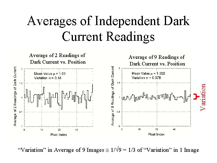
Averages of Independent Dark Current Readings Average of 9 Readings of Dark Current vs. Position Variation Average of 2 Readings of Dark Current vs. Position “Variation” in Average of 9 Images 1/ 9 = 1/3 of “Variation” in 1 Image

Infrequent Photon Arrivals • Different Mechanism – Number of Photons is an “Integer”! • Different Distribution of Values

Problem: Photon Counting Statistics • Photons from Source Arrive “Infrequently” – Few Photons • Measurement of Number of Source Photons (Also) is NOT Deterministic – Random Numbers – Distribution of Random Numbers of “Rarely Occurring” Events is Governed by Poisson Statistics

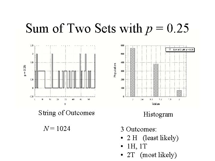
Simplest Distribution of Integers • Only Two Possible Outcomes: – YES – NO • Only One Parameter in Distribution – “Likelihood” of Outcome YES – Call it “p” – Just like Counting Coin Flips – Examples with 1024 Flips of a Coin

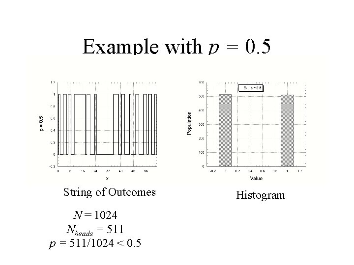
Example with p = 0. 5 String of Outcomes N = 1024 Nheads = 511 p = 511/1024 < 0. 5 Histogram

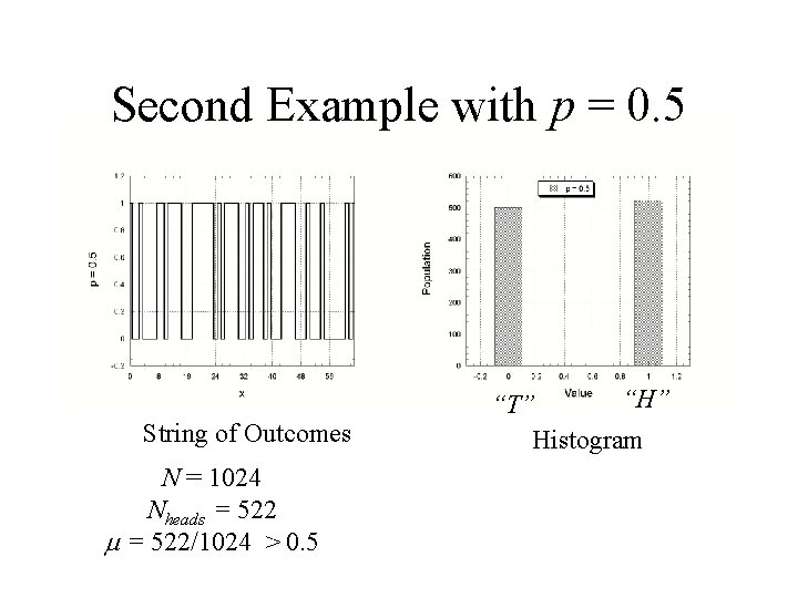
Second Example with p = 0. 5 String of Outcomes N = 1024 Nheads = 522/1024 > 0. 5 “H” “T” Histogram

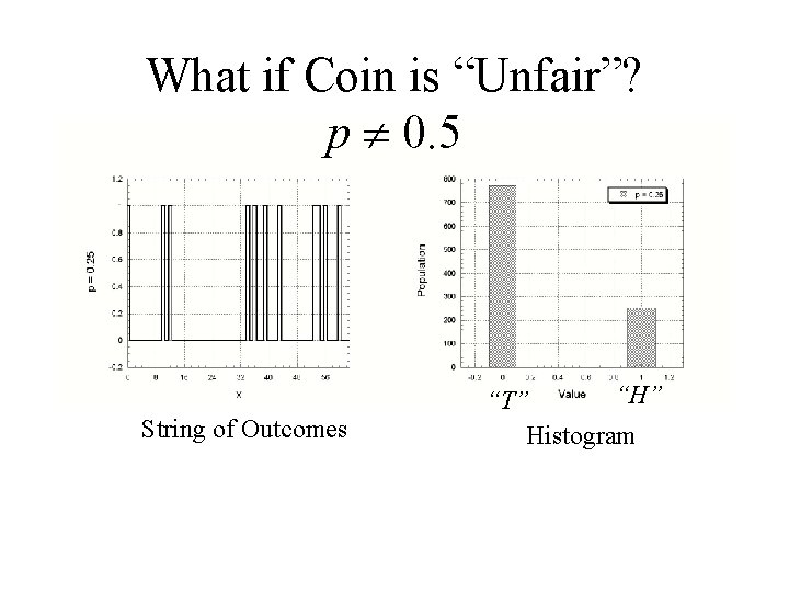
What if Coin is “Unfair”? p 0. 5 String of Outcomes “H” “T” Histogram

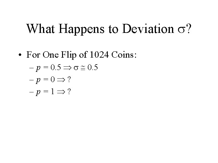
What Happens to Deviation ? • For One Flip of 1024 Coins: – p = 0. 5 –p=0 ? –p=1 ?

Deviation is Largest if p = 0. 5! • The Possible Variation is Largest if p is in the middle!

Add More “Tosses” • 2 Coin Tosses More Possibilities for Photon Arrivals

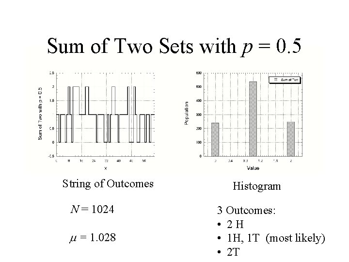
Sum of Two Sets with p = 0. 5 String of Outcomes N = 1024 = 1. 028 Histogram 3 Outcomes: • 2 H • 1 H, 1 T (most likely) • 2 T

Sum of Two Sets with p = 0. 25 String of Outcomes N = 1024 Histogram 3 Outcomes: • 2 H (least likely) • 1 H, 1 T • 2 T (most likely)

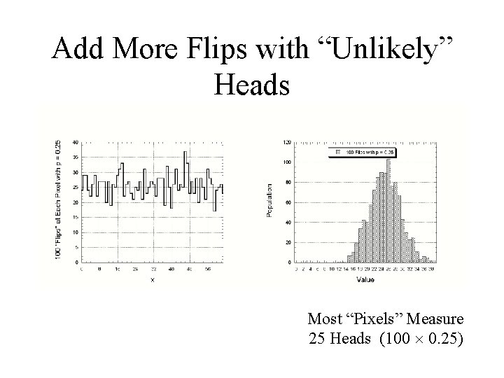
Add More Flips with “Unlikely” Heads Most “Pixels” Measure 25 Heads (100 0. 25)

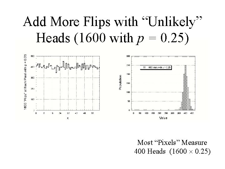
Add More Flips with “Unlikely” Heads (1600 with p = 0. 25) Most “Pixels” Measure 400 Heads (1600 0. 25)

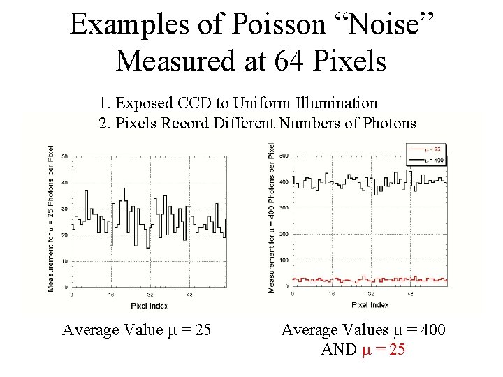
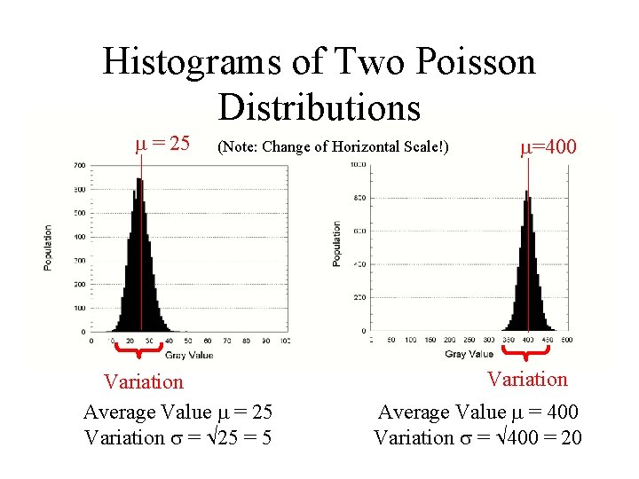
Examples of Poisson “Noise” Measured at 64 Pixels 1. Exposed CCD to Uniform Illumination 2. Pixels Record Different Numbers of Photons Average Value = 25 Average Values = 400 AND = 25

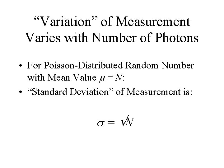
“Variation” of Measurement Varies with Number of Photons • For Poisson-Distributed Random Number with Mean Value = N: • “Standard Deviation” of Measurement is: = N

Histograms of Two Poisson Distributions = 25 (Note: Change of Horizontal Scale!) Variation Average Value = 25 Variation = 25 = 5 =400 Variation Average Value = 400 Variation = 400 = 20

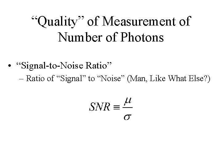
“Quality” of Measurement of Number of Photons • “Signal-to-Noise Ratio” – Ratio of “Signal” to “Noise” (Man, Like What Else? )

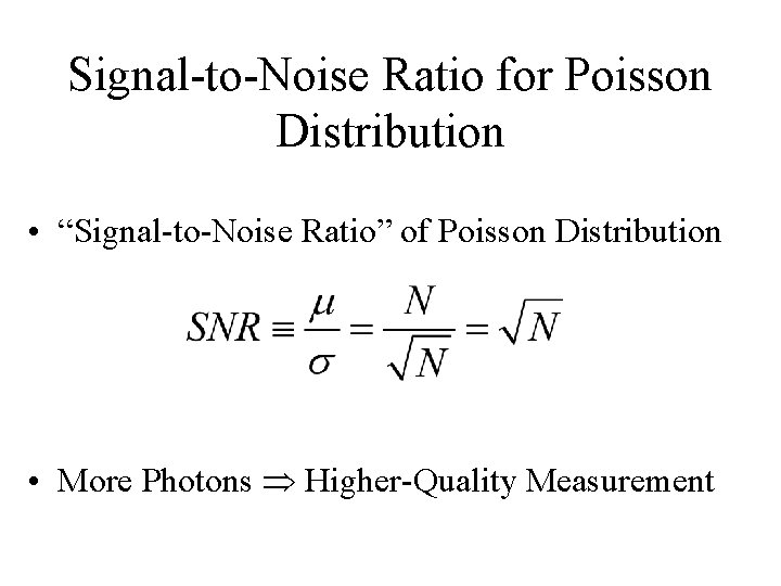
Signal-to-Noise Ratio for Poisson Distribution • “Signal-to-Noise Ratio” of Poisson Distribution • More Photons Higher-Quality Measurement

Solution: Photon Counting Statistics • Collect as MANY Photons as POSSIBLE!! • Largest Aperture (Telescope Collecting Area) • Longest Exposure Time • Maximizes Source Illumination on Detector – Increases Number of Photons • Issue is More Important for X Rays than for Longer Wavelengths – Fewer X-Ray Photons

Problem: Read Noise • Uncertainty in Number of Electrons Counted – Due to Statistical Errors, Just Like Photon Counts • Detector Electronics

Solution: Read Noise • Collect Sufficient Number of Photons so that Read Noise is Less Important Than Photon Counting Noise • Some Electronic Sensors (CCD-“like” Devices) Can Be Read Out “Nondestructively” – “Charge Injection Devices” (CIDs) – Used in Infrared • multiple reads of CID pixels reduces uncertainty

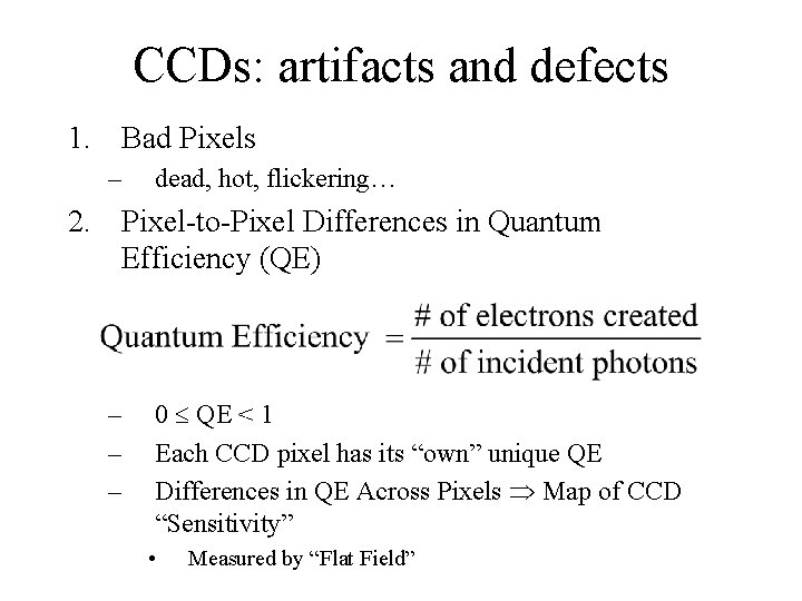
CCDs: artifacts and defects 1. Bad Pixels – dead, hot, flickering… 2. Pixel-to-Pixel Differences in Quantum Efficiency (QE) – – – 0 QE < 1 Each CCD pixel has its “own” unique QE Differences in QE Across Pixels Map of CCD “Sensitivity” • Measured by “Flat Field”

CCDs: artifacts and defects 3. Saturation – each pixel can hold a limited quantity of electrons (limited well depth of a pixel) 4. Loss of Charge during pixel charge transfer & readout – Pixel’s Value at Readout May Not Be What Was Measured When Light Was Collected

Bad Pixels • Issue: Some Fraction of Pixels in a CCD are: – “Dead” (measure no charge) – “Hot” (always measure more charge than collected) • Solutions: – Replace Value of Bad Pixel with Average of Pixel’s Neighbors – Dither the Telescope over a Series of Images • Move Telescope Slightly Between Images to Ensure that Source Fall on Good Pixels in Some of the Images • Different Images Must be “Registered” (Aligned) and Appropriately Combined

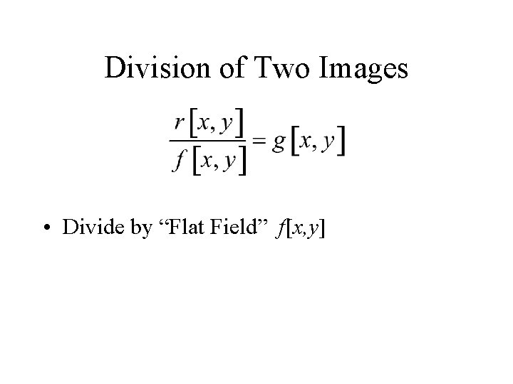
Pixel-to-Pixel Differences in QE • Issue: each pixel has its own response to light • Solution: obtain and use a flat field image to correct for pixel-to-pixel nonuniformities – construct flat field by exposing CCD to a uniform source of illumination • image the sky or a white screen pasted on the dome – divide source images by the flat field image • for every pixel x, y, new source intensity is now S’(x, y) = S(x, y)/F(x, y) where F(x, y) is the flat field pixel value; “bright” pixels are suppressed, “dim” pixels are emphasized

Issue: Saturation • Issue: each pixel can only hold so many electrons (limited well depth of the pixel), so image of bright source often saturates detector – at saturation, pixel stops detecting new photons (like overexposure) – saturated pixels can “bleed” over to neighbors, causing streaks in image • Solution: put less light on detector in each image – take shorter exposures and add them together • telescope pointing will drift; need to re-register images • read noise can become a problem – use neutral density filter • a filter that blocks some light at all wavelengths uniformly • fainter sources lost

Solution to Saturation • Reduce Light on Detector in Each Image – Take a Series of Shorter Exposures and Add Them Together • Telescope Usually “Drifts” – Images Must be “Re-Registered” • Read Noise Worsens – Use Neutral Density Filter • Blocks Same Percentage of Light at All Wavelengths • Fainter Sources Lost

Issue: Loss of Electron Charge • No CCD Transfers Charge Between Pixels with 100% Efficiency – Introduces Uncertainty in Converting to Light Intensity (of “Optical” Visible Light) or to Photon Energy (for X Rays)

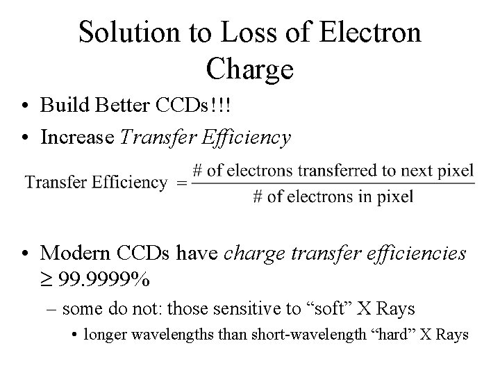
Solution to Loss of Electron Charge • Build Better CCDs!!! • Increase Transfer Efficiency • Modern CCDs have charge transfer efficiencies 99. 9999% – some do not: those sensitive to “soft” X Rays • longer wavelengths than short-wavelength “hard” X Rays

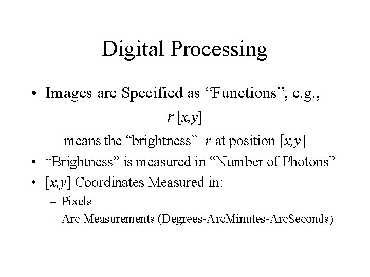
Digital Processing of Astronomical Images • Computer Processing of Digital Images • Arithmetic Calculations: – Addition – Subtraction – Multiplication – Division

Digital Processing • Images are Specified as “Functions”, e. g. , r [x, y] means the “brightness” r at position [x, y] • “Brightness” is measured in “Number of Photons” • [x, y] Coordinates Measured in: – Pixels – Arc Measurements (Degrees-Arc. Minutes-Arc. Seconds)

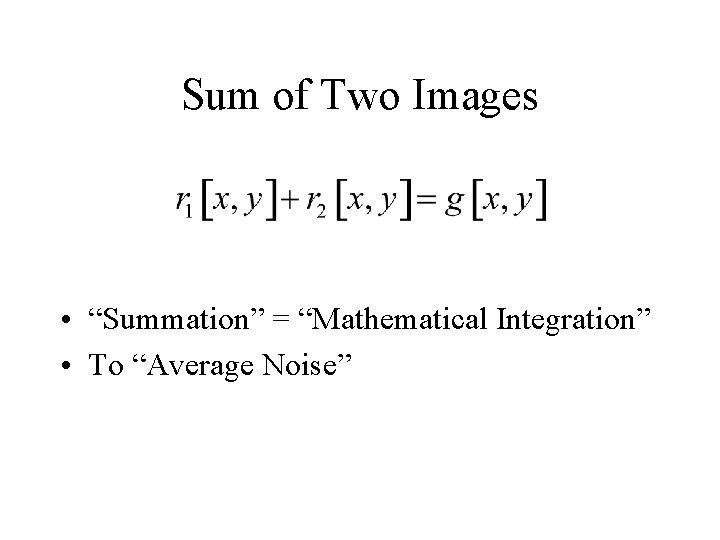
Sum of Two Images • “Summation” = “Mathematical Integration” • To “Average Noise”

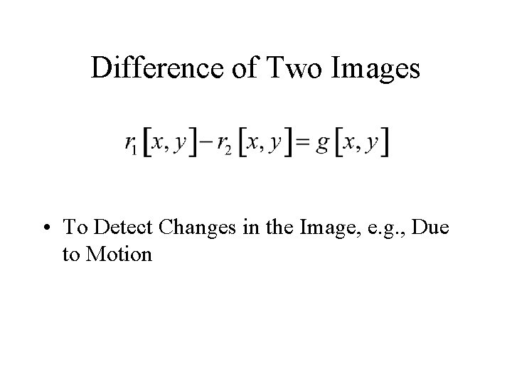
Difference of Two Images • To Detect Changes in the Image, e. g. , Due to Motion

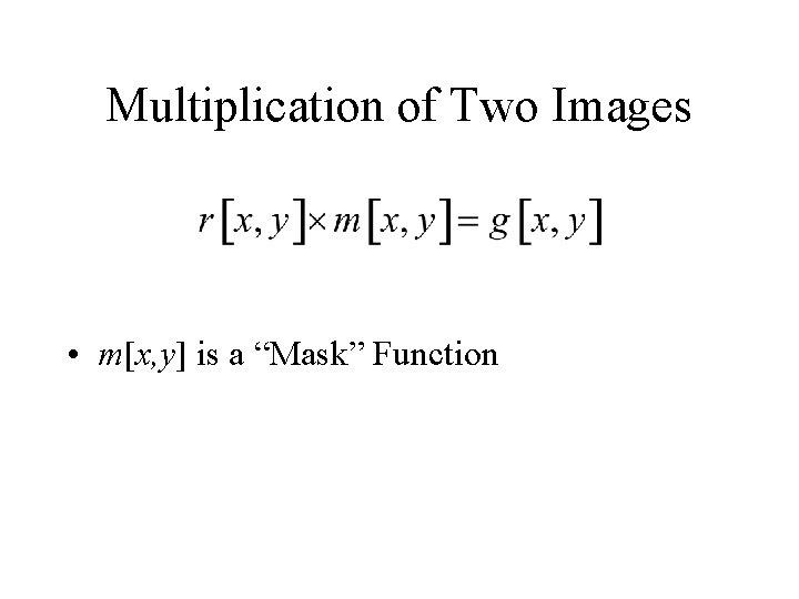
Multiplication of Two Images • m[x, y] is a “Mask” Function

Division of Two Images • Divide by “Flat Field” f[x, y]

Data Pipelining • Issue: now that I’ve collected all of these images, what do I do? • Solution: build an automated data processing pipeline – Space observatories (e. g. , HST) routinely process raw image data and deliver only the processed images to the observer – ground-based observatories are slowly coming around to this operational model – RIT’s CIS is in the “data pipeline” business • NASA’s SOFIA • South Pole facilities