Figure 10 1 Processing steps in the discretetime
![Figure 10. 11 Two segments of the linear chirp signal x[n] = cos(α 0 Figure 10. 11 Two segments of the linear chirp signal x[n] = cos(α 0](https://slidetodoc.com/presentation_image/6a5da5c32d3d4f119296b836f7f25624/image-14.jpg)
![Figure 10. 13 The magnitude of the time-dependent Fourier transform of y[n] in Eq. Figure 10. 13 The magnitude of the time-dependent Fourier transform of y[n] in Eq.](https://slidetodoc.com/presentation_image/6a5da5c32d3d4f119296b836f7f25624/image-16.jpg)

![Figure 10. 28 Computation of the circular autocorrelation. (a) x[n] and x[n + m] Figure 10. 28 Computation of the circular autocorrelation. (a) x[n] and x[n + m]](https://slidetodoc.com/presentation_image/6a5da5c32d3d4f119296b836f7f25624/image-33.jpg)
- Slides: 63

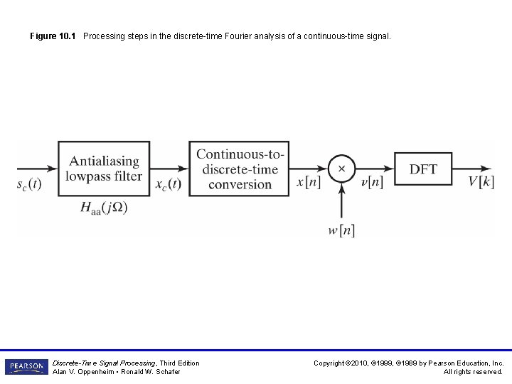
Figure 10. 1 Processing steps in the discrete-time Fourier analysis of a continuous-time signal. Discrete-Time Signal Processing, Third Edition Alan V. Oppenheim • Ronald W. Schafer Copyright © 2010, © 1999, © 1989 by Pearson Education, Inc. All rights reserved.

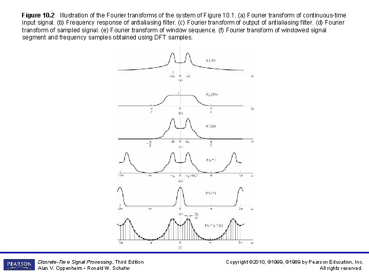
Figure 10. 2 Illustration of the Fourier transforms of the system of Figure 10. 1. (a) Fourier transform of continuous-time input signal. (b) Frequency response of antialiasing filter. (c) Fourier transform of output of antialiasing filter. (d) Fourier transform of sampled signal. (e) Fourier transform of window sequence. (f) Fourier transform of windowed signal segment and frequency samples obtained using DFT samples. Discrete-Time Signal Processing, Third Edition Alan V. Oppenheim • Ronald W. Schafer Copyright © 2010, © 1999, © 1989 by Pearson Education, Inc. All rights reserved.

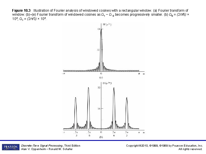
Figure 10. 3 Illustration of Fourier analysis of windowed cosines with a rectangular window. (a) Fourier transform of window. (b)–(e) Fourier transform of windowed cosines as Ω 1 − Ω 0 becomes progressively smaller. (b) Ω 0 = (2π/6) × 104, Ω 1 = (2π/3) × 104. Discrete-Time Signal Processing, Third Edition Alan V. Oppenheim • Ronald W. Schafer Copyright © 2010, © 1999, © 1989 by Pearson Education, Inc. All rights reserved.

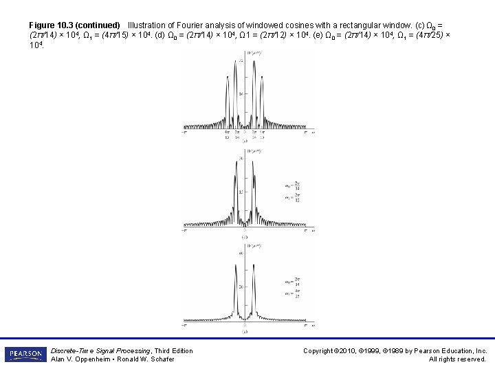
Figure 10. 3 (continued) Illustration of Fourier analysis of windowed cosines with a rectangular window. (c) Ω 0 = (2π/14) × 104, Ω 1 = (4π/15) × 104. (d) Ω 0 = (2π/14) × 104, Ω 1 = (2π/12) × 104. (e) Ω 0 = (2π/14) × 104, Ω 1 = (4π/25) × 104. Discrete-Time Signal Processing, Third Edition Alan V. Oppenheim • Ronald W. Schafer Copyright © 2010, © 1999, © 1989 by Pearson Education, Inc. All rights reserved.

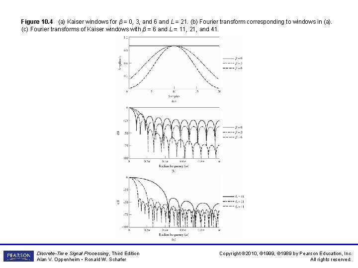
Figure 10. 4 (a) Kaiser windows for β = 0, 3, and 6 and L = 21. (b) Fourier transform corresponding to windows in (a). (c) Fourier transforms of Kaiser windows with β = 6 and L = 11, 21, and 41. Discrete-Time Signal Processing, Third Edition Alan V. Oppenheim • Ronald W. Schafer Copyright © 2010, © 1999, © 1989 by Pearson Education, Inc. All rights reserved.

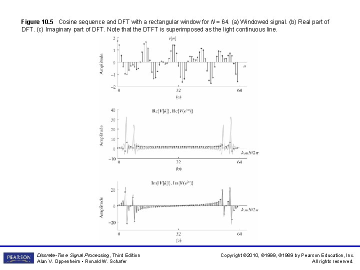
Figure 10. 5 Cosine sequence and DFT with a rectangular window for N = 64. (a) Windowed signal. (b) Real part of DFT. (c) Imaginary part of DFT. Note that the DTFT is superimposed as the light continuous line. Discrete-Time Signal Processing, Third Edition Alan V. Oppenheim • Ronald W. Schafer Copyright © 2010, © 1999, © 1989 by Pearson Education, Inc. All rights reserved.

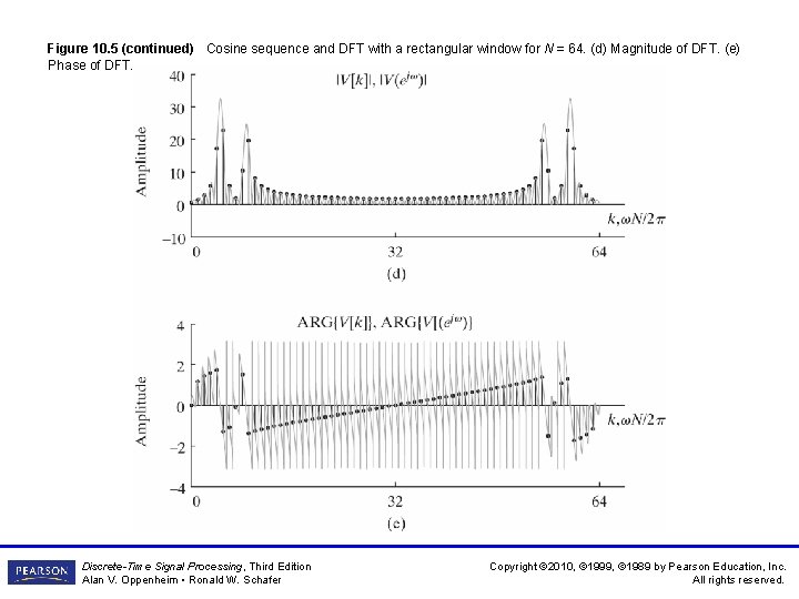
Figure 10. 5 (continued) Cosine sequence and DFT with a rectangular window for N = 64. (d) Magnitude of DFT. (e) Phase of DFT. Discrete-Time Signal Processing, Third Edition Alan V. Oppenheim • Ronald W. Schafer Copyright © 2010, © 1999, © 1989 by Pearson Education, Inc. All rights reserved.

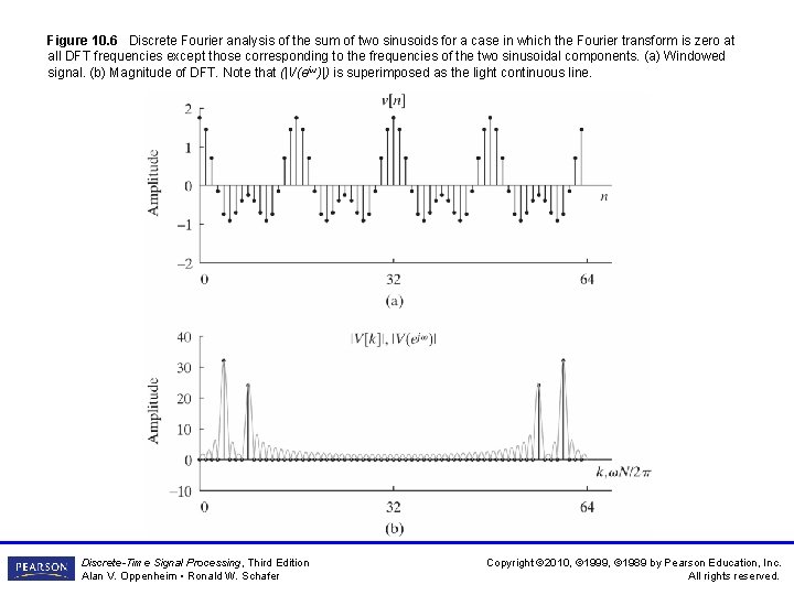
Figure 10. 6 Discrete Fourier analysis of the sum of two sinusoids for a case in which the Fourier transform is zero at all DFT frequencies except those corresponding to the frequencies of the two sinusoidal components. (a) Windowed signal. (b) Magnitude of DFT. Note that (|V(ejω)|) is superimposed as the light continuous line. Discrete-Time Signal Processing, Third Edition Alan V. Oppenheim • Ronald W. Schafer Copyright © 2010, © 1999, © 1989 by Pearson Education, Inc. All rights reserved.

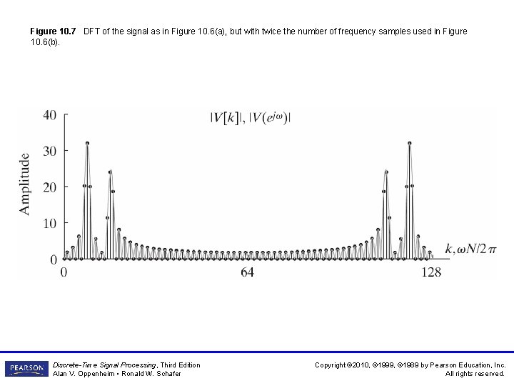
Figure 10. 7 DFT of the signal as in Figure 10. 6(a), but with twice the number of frequency samples used in Figure 10. 6(b). Discrete-Time Signal Processing, Third Edition Alan V. Oppenheim • Ronald W. Schafer Copyright © 2010, © 1999, © 1989 by Pearson Education, Inc. All rights reserved.

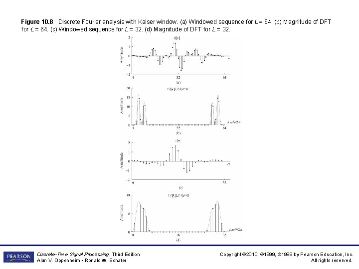
Figure 10. 8 Discrete Fourier analysis with Kaiser window. (a) Windowed sequence for L = 64. (b) Magnitude of DFT for L = 64. (c) Windowed sequence for L = 32. (d) Magnitude of DFT for L = 32. Discrete-Time Signal Processing, Third Edition Alan V. Oppenheim • Ronald W. Schafer Copyright © 2010, © 1999, © 1989 by Pearson Education, Inc. All rights reserved.

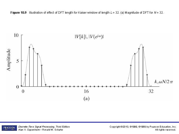
Figure 10. 9 Illustration of effect of DFT length for Kaiser window of length L = 32. (a) Magnitude of DFT for N = 32. Discrete-Time Signal Processing, Third Edition Alan V. Oppenheim • Ronald W. Schafer Copyright © 2010, © 1999, © 1989 by Pearson Education, Inc. All rights reserved.

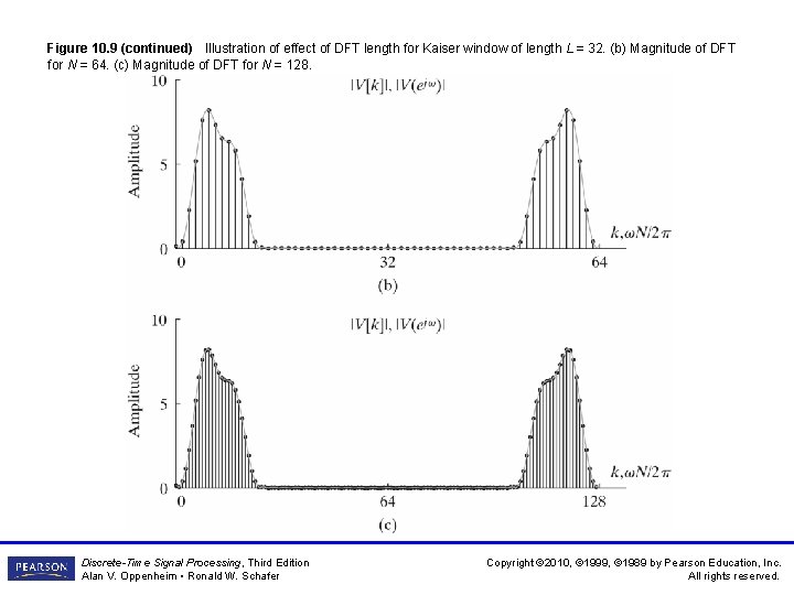
Figure 10. 9 (continued) Illustration of effect of DFT length for Kaiser window of length L = 32. (b) Magnitude of DFT for N = 64. (c) Magnitude of DFT for N = 128. Discrete-Time Signal Processing, Third Edition Alan V. Oppenheim • Ronald W. Schafer Copyright © 2010, © 1999, © 1989 by Pearson Education, Inc. All rights reserved.

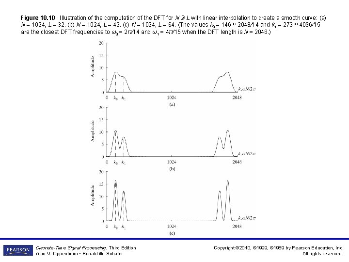
Figure 10. 10 Illustration of the computation of the DFT for N » L with linear interpolation to create a smooth curve: (a) N = 1024, L = 32. (b) N = 1024, L = 42. (c) N = 1024, L = 64. (The values k 0 = 146 ≈ 2048/14 and k 1 = 273 ≈ 4096/15 are the closest DFT frequencies to ω0 = 2π/14 and ω1 = 4π/15 when the DFT length is N = 2048. ) Discrete-Time Signal Processing, Third Edition Alan V. Oppenheim • Ronald W. Schafer Copyright © 2010, © 1999, © 1989 by Pearson Education, Inc. All rights reserved.
![Figure 10 11 Two segments of the linear chirp signal xn cosα 0 Figure 10. 11 Two segments of the linear chirp signal x[n] = cos(α 0](https://slidetodoc.com/presentation_image/6a5da5c32d3d4f119296b836f7f25624/image-14.jpg)
Figure 10. 11 Two segments of the linear chirp signal x[n] = cos(α 0 n 2) for α 0 = 15π× 10− 6 with a 400 -sample Hamming window superimposed. (a) X[n, λ) at n = 320 would be the DTFT of the top trace multiplied by the window. (b) X[720, λ) would be the DTFT of the bottom trace multiplied by the window. Discrete-Time Signal Processing, Third Edition Alan V. Oppenheim • Ronald W. Schafer Copyright © 2010, © 1999, © 1989 by Pearson Education, Inc. All rights reserved.

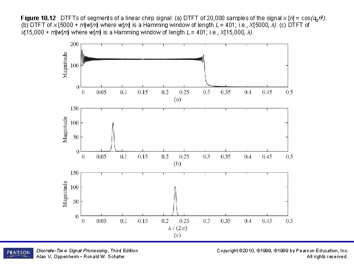
Figure 10. 12 DTFTs of segments of a linear chirp signal: (a) DTFT of 20, 000 samples of the signal x [n] = cos(α 0 n 2). (b) DTFT of x [5000 + m]w[m] where w[m] is a Hamming window of length L = 401; i. e. , X[5000, λ). (c) DTFT of x[15, 000 + m]w[m] where w[m] is a Hamming window of length L = 401; i. e. , X[15, 000, λ). Discrete-Time Signal Processing, Third Edition Alan V. Oppenheim • Ronald W. Schafer Copyright © 2010, © 1999, © 1989 by Pearson Education, Inc. All rights reserved.
![Figure 10 13 The magnitude of the timedependent Fourier transform of yn in Eq Figure 10. 13 The magnitude of the time-dependent Fourier transform of y[n] in Eq.](https://slidetodoc.com/presentation_image/6a5da5c32d3d4f119296b836f7f25624/image-16.jpg)
Figure 10. 13 The magnitude of the time-dependent Fourier transform of y[n] in Eq. (10. 23): (a) Using a Hamming window of length L = 401. (b) Using a Hamming window of length L = 101. Discrete-Time Signal Processing, Third Edition Alan V. Oppenheim • Ronald W. Schafer Copyright © 2010, © 1999, © 1989 by Pearson Education, Inc. All rights reserved.

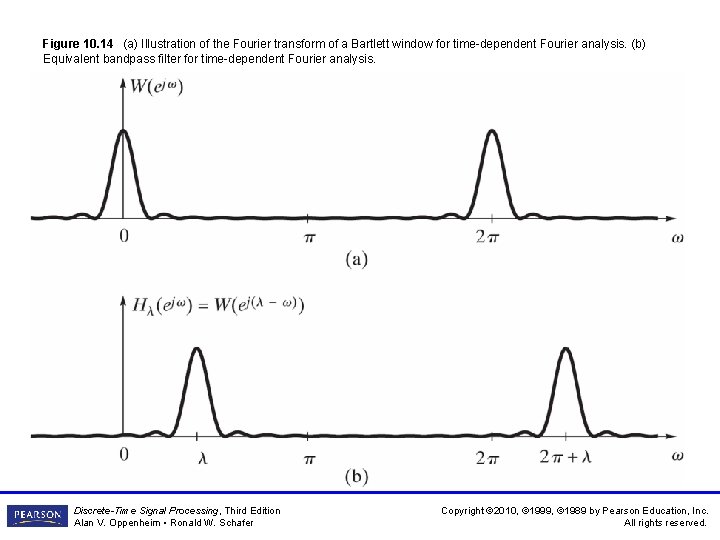
Figure 10. 14 (a) Illustration of the Fourier transform of a Bartlett window for time-dependent Fourier analysis. (b) Equivalent bandpass filter for time-dependent Fourier analysis. Discrete-Time Signal Processing, Third Edition Alan V. Oppenheim • Ronald W. Schafer Copyright © 2010, © 1999, © 1989 by Pearson Education, Inc. All rights reserved.

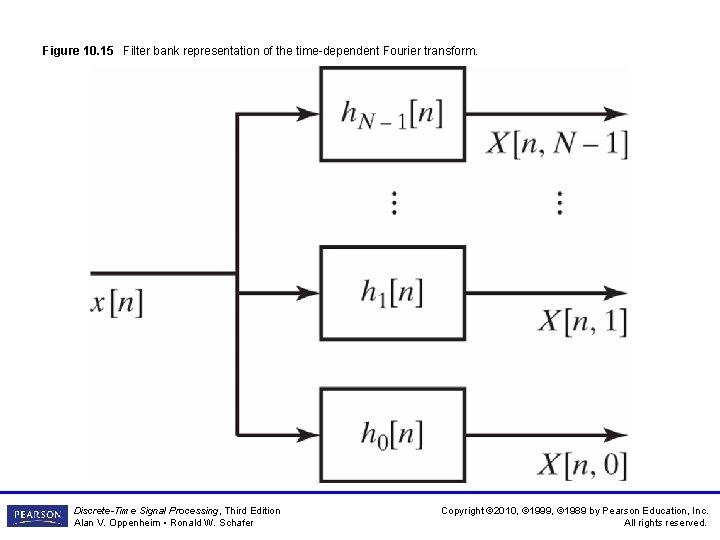
Figure 10. 15 Filter bank representation of the time-dependent Fourier transform. Discrete-Time Signal Processing, Third Edition Alan V. Oppenheim • Ronald W. Schafer Copyright © 2010, © 1999, © 1989 by Pearson Education, Inc. All rights reserved.

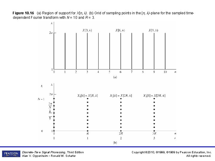
Figure 10. 16 (a) Region of support for X[n, λ). (b) Grid of sampling points in the [n, λ)-plane for the sampled timedependent Fourier transform with N = 10 and R = 3. Discrete-Time Signal Processing, Third Edition Alan V. Oppenheim • Ronald W. Schafer Copyright © 2010, © 1999, © 1989 by Pearson Education, Inc. All rights reserved.

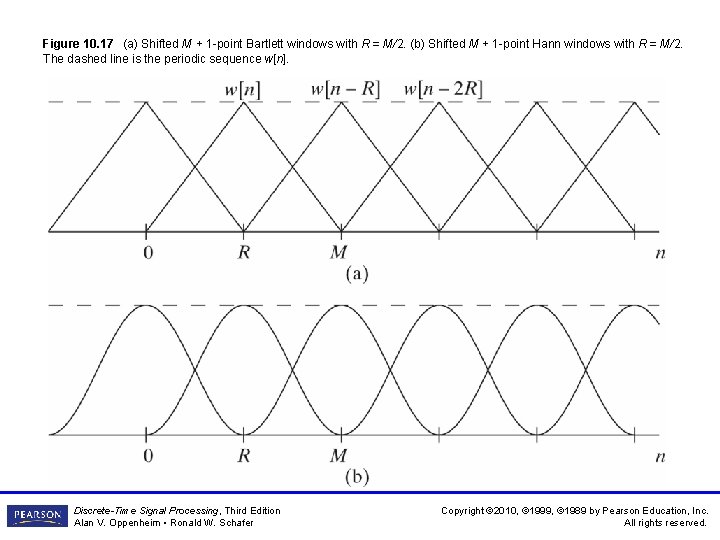
Figure 10. 17 (a) Shifted M + 1 -point Bartlett windows with R = M/2. (b) Shifted M + 1 -point Hann windows with R = M/2. The dashed line is the periodic sequence w[n]. Discrete-Time Signal Processing, Third Edition Alan V. Oppenheim • Ronald W. Schafer Copyright © 2010, © 1999, © 1989 by Pearson Education, Inc. All rights reserved.

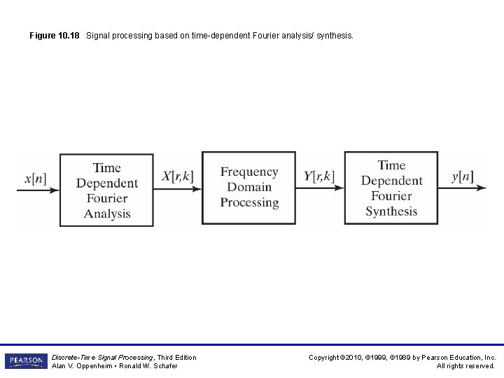
Figure 10. 18 Signal processing based on time-dependent Fourier analysis/ synthesis. Discrete-Time Signal Processing, Third Edition Alan V. Oppenheim • Ronald W. Schafer Copyright © 2010, © 1999, © 1989 by Pearson Education, Inc. All rights reserved.

Figure 10. 19 Filterbank frequency response. (a) Rectangular window. (b) Kaiser window. Discrete-Time Signal Processing, Third Edition Alan V. Oppenheim • Ronald W. Schafer Copyright © 2010, © 1999, © 1989 by Pearson Education, Inc. All rights reserved.

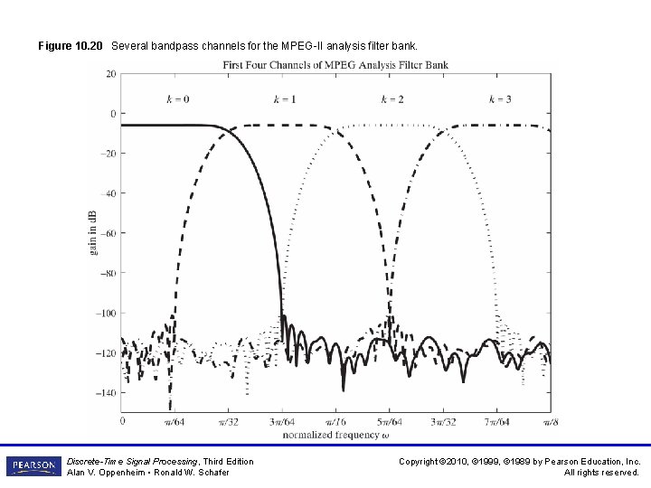
Figure 10. 20 Several bandpass channels for the MPEG-II analysis filter bank. Discrete-Time Signal Processing, Third Edition Alan V. Oppenheim • Ronald W. Schafer Copyright © 2010, © 1999, © 1989 by Pearson Education, Inc. All rights reserved.

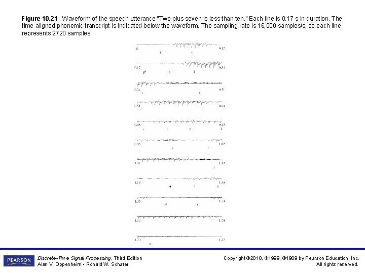
Figure 10. 21 Waveform of the speech utterance “Two plus seven is less than ten. ” Each line is 0. 17 s in duration. The time-aligned phonemic transcript is indicated below the waveform. The sampling rate is 16, 000 samples/s, so each line represents 2720 samples. Discrete-Time Signal Processing, Third Edition Alan V. Oppenheim • Ronald W. Schafer Copyright © 2010, © 1999, © 1989 by Pearson Education, Inc. All rights reserved.

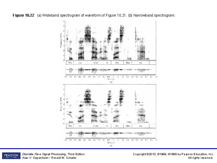
Figure 10. 22 (a) Wideband spectrogram of waveform of Figure 10. 21. (b) Narrowband spectrogram. Discrete-Time Signal Processing, Third Edition Alan V. Oppenheim • Ronald W. Schafer Copyright © 2010, © 1999, © 1989 by Pearson Education, Inc. All rights reserved.

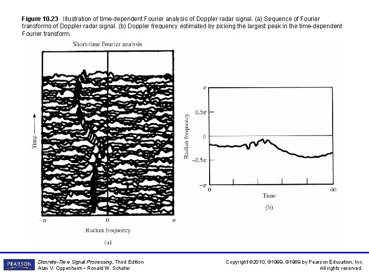
Figure 10. 23 Illustration of time-dependent Fourier analysis of Doppler radar signal. (a) Sequence of Fourier transforms of Doppler radar signal. (b) Doppler frequency estimated by picking the largest peak in the time-dependent Fourier transform. Discrete-Time Signal Processing, Third Edition Alan V. Oppenheim • Ronald W. Schafer Copyright © 2010, © 1999, © 1989 by Pearson Education, Inc. All rights reserved.

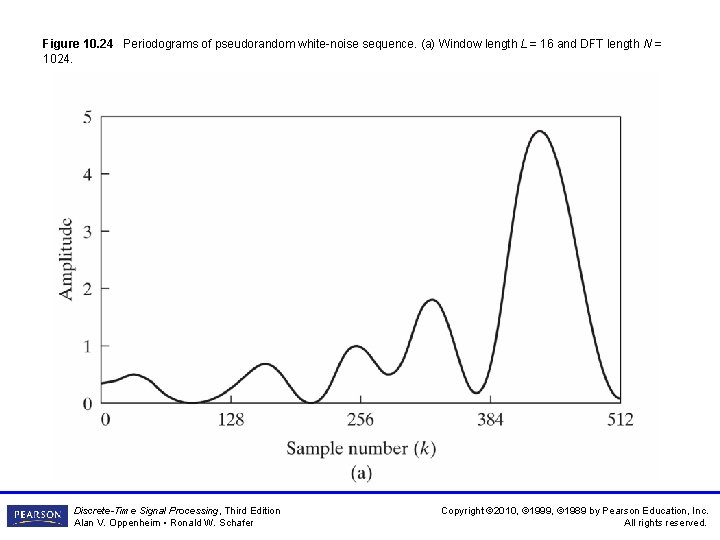
Figure 10. 24 Periodograms of pseudorandom white-noise sequence. (a) Window length L = 16 and DFT length N = 1024. Discrete-Time Signal Processing, Third Edition Alan V. Oppenheim • Ronald W. Schafer Copyright © 2010, © 1999, © 1989 by Pearson Education, Inc. All rights reserved.

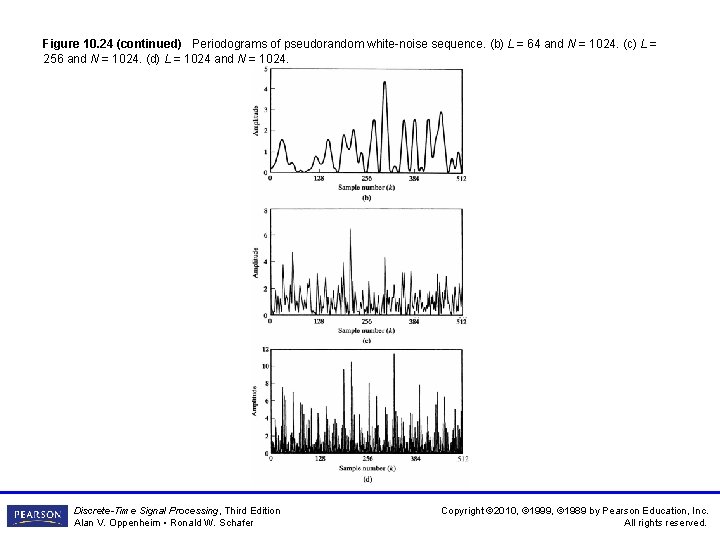
Figure 10. 24 (continued) Periodograms of pseudorandom white-noise sequence. (b) L = 64 and N = 1024. (c) L = 256 and N = 1024. (d) L = 1024 and N = 1024. Discrete-Time Signal Processing, Third Edition Alan V. Oppenheim • Ronald W. Schafer Copyright © 2010, © 1999, © 1989 by Pearson Education, Inc. All rights reserved.

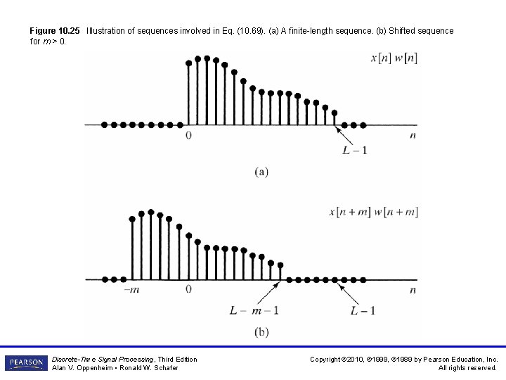
Figure 10. 25 Illustration of sequences involved in Eq. (10. 69). (a) A finite-length sequence. (b) Shifted sequence for m > 0. Discrete-Time Signal Processing, Third Edition Alan V. Oppenheim • Ronald W. Schafer Copyright © 2010, © 1999, © 1989 by Pearson Education, Inc. All rights reserved.

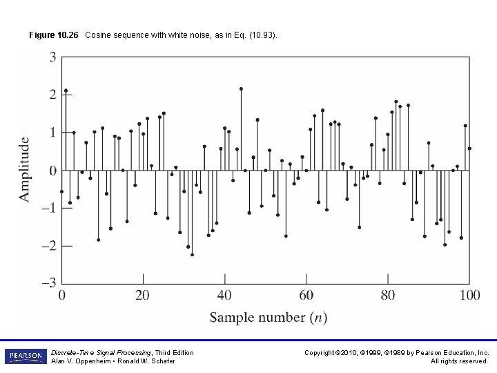
Figure 10. 26 Cosine sequence with white noise, as in Eq. (10. 93). Discrete-Time Signal Processing, Third Edition Alan V. Oppenheim • Ronald W. Schafer Copyright © 2010, © 1999, © 1989 by Pearson Education, Inc. All rights reserved.

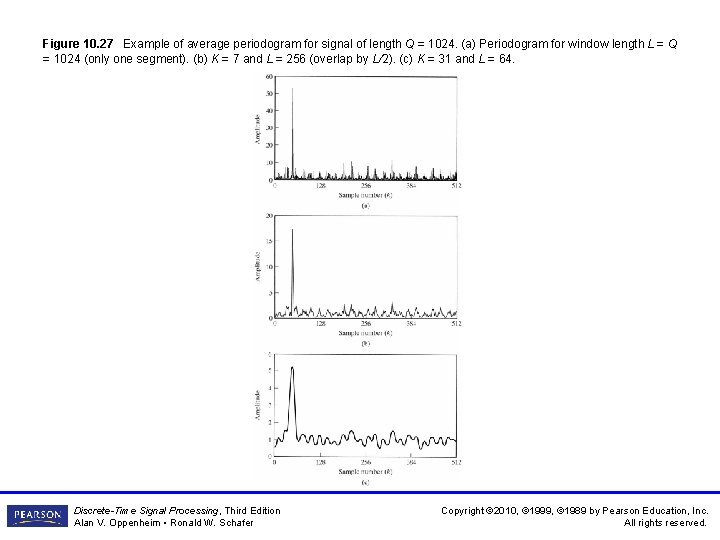
Figure 10. 27 Example of average periodogram for signal of length Q = 1024. (a) Periodogram for window length L = Q = 1024 (only one segment). (b) K = 7 and L = 256 (overlap by L/2). (c) K = 31 and L = 64. Discrete-Time Signal Processing, Third Edition Alan V. Oppenheim • Ronald W. Schafer Copyright © 2010, © 1999, © 1989 by Pearson Education, Inc. All rights reserved.

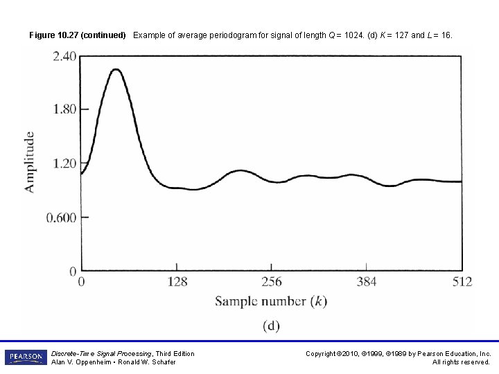
Figure 10. 27 (continued) Example of average periodogram for signal of length Q = 1024. (d) K = 127 and L = 16. Discrete-Time Signal Processing, Third Edition Alan V. Oppenheim • Ronald W. Schafer Copyright © 2010, © 1999, © 1989 by Pearson Education, Inc. All rights reserved.
![Figure 10 28 Computation of the circular autocorrelation a xn and xn m Figure 10. 28 Computation of the circular autocorrelation. (a) x[n] and x[n + m]](https://slidetodoc.com/presentation_image/6a5da5c32d3d4f119296b836f7f25624/image-33.jpg)
Figure 10. 28 Computation of the circular autocorrelation. (a) x[n] and x[n + m] for a finite-length sequence of length Q. (b) x [n] and x [((n + m))N ] as in circular correlation. Discrete-Time Signal Processing, Third Edition Alan V. Oppenheim • Ronald W. Schafer Copyright © 2010, © 1999, © 1989 by Pearson Education, Inc. All rights reserved.

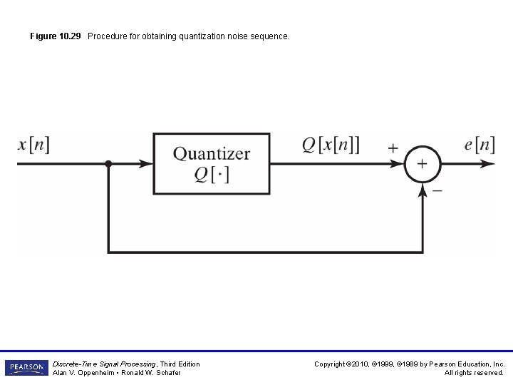
Figure 10. 29 Procedure for obtaining quantization noise sequence. Discrete-Time Signal Processing, Third Edition Alan V. Oppenheim • Ronald W. Schafer Copyright © 2010, © 1999, © 1989 by Pearson Education, Inc. All rights reserved.

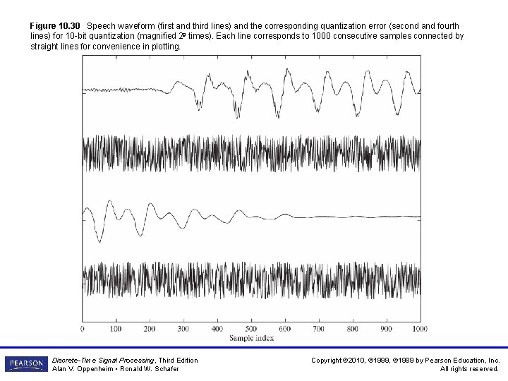
Figure 10. 30 Speech waveform (first and third lines) and the corresponding quantization error (second and fourth lines) for 10 -bit quantization (magnified 29 times). Each line corresponds to 1000 consecutive samples connected by straight lines for convenience in plotting. Discrete-Time Signal Processing, Third Edition Alan V. Oppenheim • Ronald W. Schafer Copyright © 2010, © 1999, © 1989 by Pearson Education, Inc. All rights reserved.

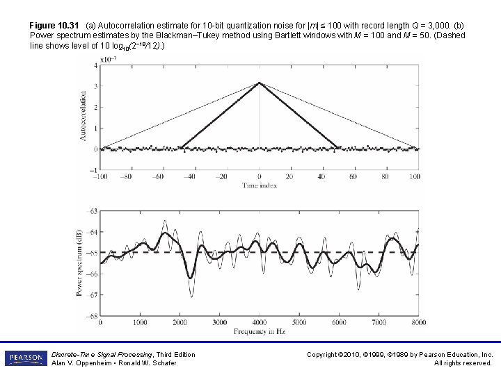
Figure 10. 31 (a) Autocorrelation estimate for 10 -bit quantization noise for |m| ≤ 100 with record length Q = 3, 000. (b) Power spectrum estimates by the Blackman–Tukey method using Bartlett windows with M = 100 and M = 50. (Dashed line shows level of 10 log 10(2− 18/12). ) Discrete-Time Signal Processing, Third Edition Alan V. Oppenheim • Ronald W. Schafer Copyright © 2010, © 1999, © 1989 by Pearson Education, Inc. All rights reserved.

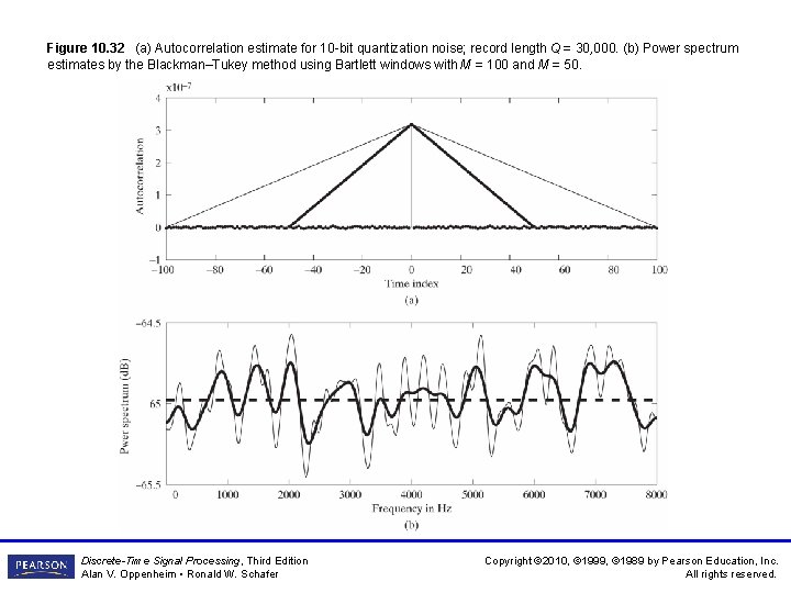
Figure 10. 32 (a) Autocorrelation estimate for 10 -bit quantization noise; record length Q = 30, 000. (b) Power spectrum estimates by the Blackman–Tukey method using Bartlett windows with M = 100 and M = 50. Discrete-Time Signal Processing, Third Edition Alan V. Oppenheim • Ronald W. Schafer Copyright © 2010, © 1999, © 1989 by Pearson Education, Inc. All rights reserved.

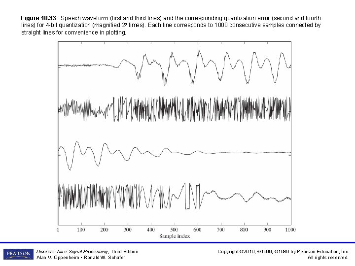
Figure 10. 33 Speech waveform (first and third lines) and the corresponding quantization error (second and fourth lines) for 4 -bit quantization (magnified 23 times). Each line corresponds to 1000 consecutive samples connected by straight lines for convenience in plotting. Discrete-Time Signal Processing, Third Edition Alan V. Oppenheim • Ronald W. Schafer Copyright © 2010, © 1999, © 1989 by Pearson Education, Inc. All rights reserved.

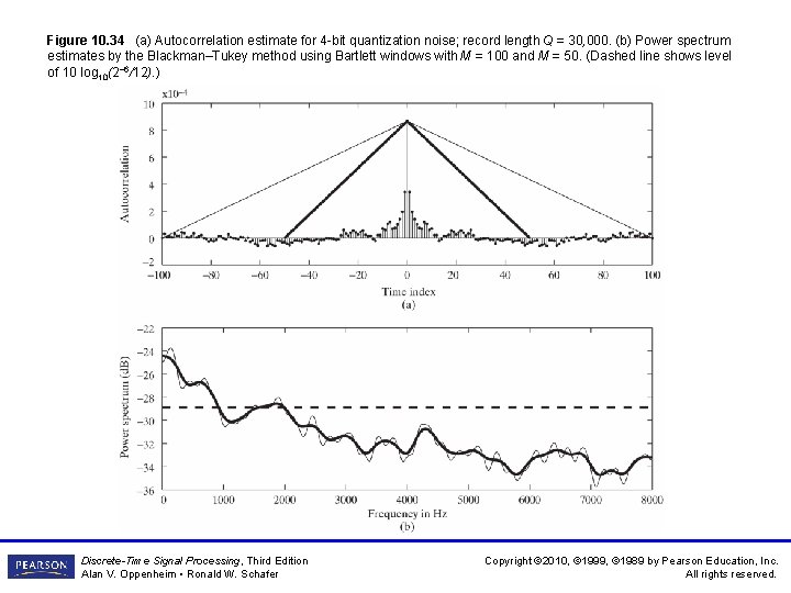
Figure 10. 34 (a) Autocorrelation estimate for 4 -bit quantization noise; record length Q = 30, 000. (b) Power spectrum estimates by the Blackman–Tukey method using Bartlett windows with M = 100 and M = 50. (Dashed line shows level of 10 log 10(2− 6/12). ) Discrete-Time Signal Processing, Third Edition Alan V. Oppenheim • Ronald W. Schafer Copyright © 2010, © 1999, © 1989 by Pearson Education, Inc. All rights reserved.

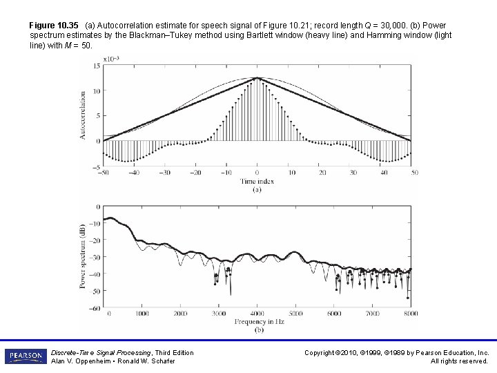
Figure 10. 35 (a) Autocorrelation estimate for speech signal of Figure 10. 21; record length Q = 30, 000. (b) Power spectrum estimates by the Blackman–Tukey method using Bartlett window (heavy line) and Hamming window (light line) with M = 50. Discrete-Time Signal Processing, Third Edition Alan V. Oppenheim • Ronald W. Schafer Copyright © 2010, © 1999, © 1989 by Pearson Education, Inc. All rights reserved.

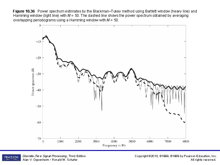
Figure 10. 36 Power spectrum estimates by the Blackman–Tukey method using Bartlett window (heavy line) and Hamming window (light line) with M = 50. The dashed line shows the power spectrum obtained by averaging overlapping periodograms using a Hamming window with M = 50. Discrete-Time Signal Processing, Third Edition Alan V. Oppenheim • Ronald W. Schafer Copyright © 2010, © 1999, © 1989 by Pearson Education, Inc. All rights reserved.

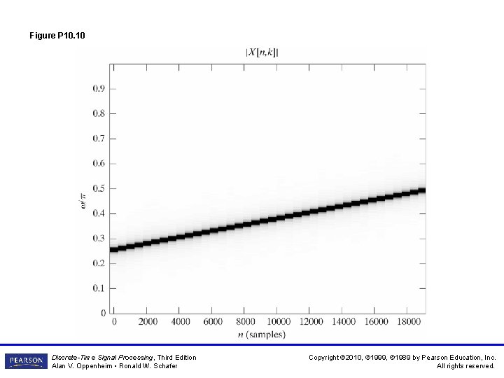
Figure P 10. 10 Discrete-Time Signal Processing, Third Edition Alan V. Oppenheim • Ronald W. Schafer Copyright © 2010, © 1999, © 1989 by Pearson Education, Inc. All rights reserved.

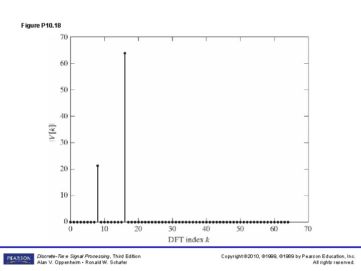
Figure P 10. 18 Discrete-Time Signal Processing, Third Edition Alan V. Oppenheim • Ronald W. Schafer Copyright © 2010, © 1999, © 1989 by Pearson Education, Inc. All rights reserved.

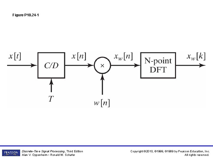
Figure P 10. 24 -1 Discrete-Time Signal Processing, Third Edition Alan V. Oppenheim • Ronald W. Schafer Copyright © 2010, © 1999, © 1989 by Pearson Education, Inc. All rights reserved.

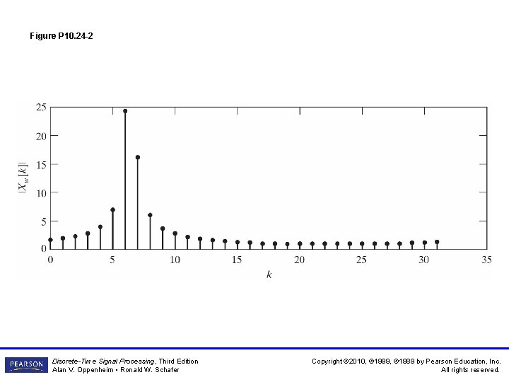
Figure P 10. 24 -2 Discrete-Time Signal Processing, Third Edition Alan V. Oppenheim • Ronald W. Schafer Copyright © 2010, © 1999, © 1989 by Pearson Education, Inc. All rights reserved.

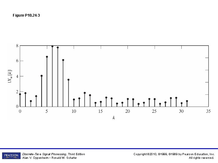
Figure P 10. 24 -3 Discrete-Time Signal Processing, Third Edition Alan V. Oppenheim • Ronald W. Schafer Copyright © 2010, © 1999, © 1989 by Pearson Education, Inc. All rights reserved.

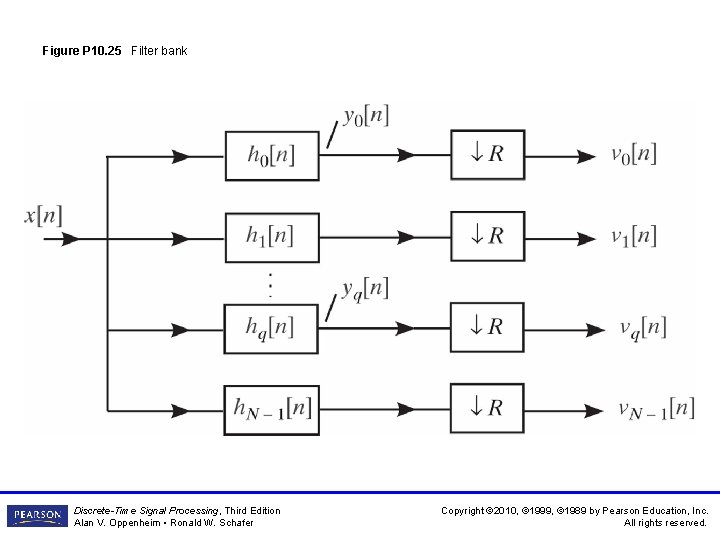
Figure P 10. 25 Filter bank Discrete-Time Signal Processing, Third Edition Alan V. Oppenheim • Ronald W. Schafer Copyright © 2010, © 1999, © 1989 by Pearson Education, Inc. All rights reserved.

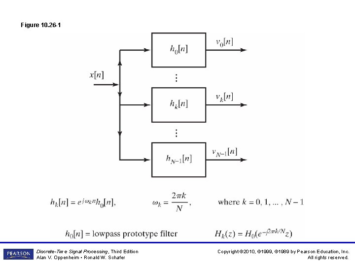
Figure 10. 26 -1 Discrete-Time Signal Processing, Third Edition Alan V. Oppenheim • Ronald W. Schafer Copyright © 2010, © 1999, © 1989 by Pearson Education, Inc. All rights reserved.

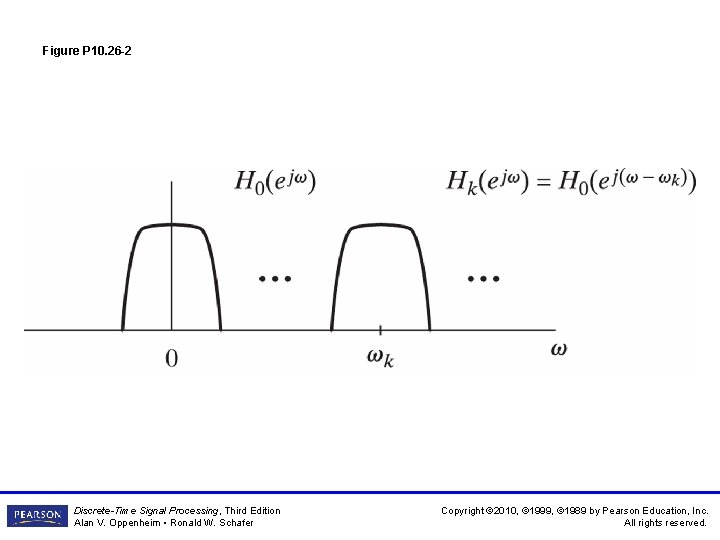
Figure P 10. 26 -2 Discrete-Time Signal Processing, Third Edition Alan V. Oppenheim • Ronald W. Schafer Copyright © 2010, © 1999, © 1989 by Pearson Education, Inc. All rights reserved.

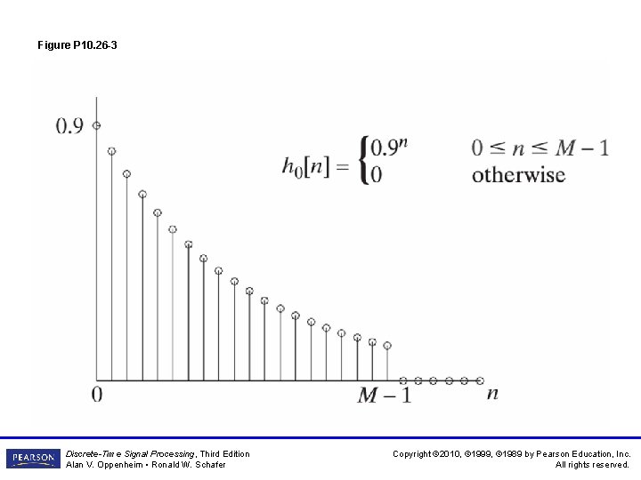
Figure P 10. 26 -3 Discrete-Time Signal Processing, Third Edition Alan V. Oppenheim • Ronald W. Schafer Copyright © 2010, © 1999, © 1989 by Pearson Education, Inc. All rights reserved.

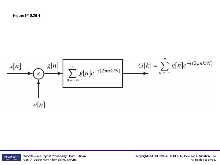
Figure P 10. 26 -4 Discrete-Time Signal Processing, Third Edition Alan V. Oppenheim • Ronald W. Schafer Copyright © 2010, © 1999, © 1989 by Pearson Education, Inc. All rights reserved.

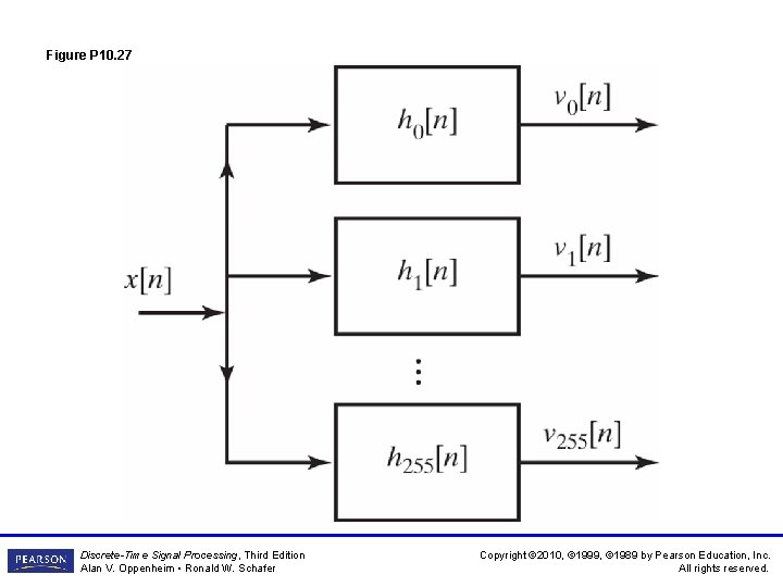
Figure P 10. 27 Discrete-Time Signal Processing, Third Edition Alan V. Oppenheim • Ronald W. Schafer Copyright © 2010, © 1999, © 1989 by Pearson Education, Inc. All rights reserved.

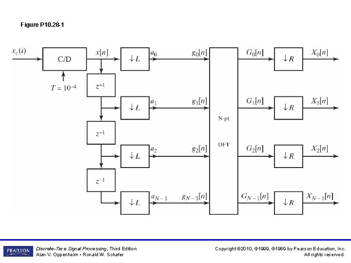
Figure P 10. 28 -1 Discrete-Time Signal Processing, Third Edition Alan V. Oppenheim • Ronald W. Schafer Copyright © 2010, © 1999, © 1989 by Pearson Education, Inc. All rights reserved.

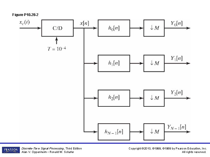
Figure P 10. 28 -2 Discrete-Time Signal Processing, Third Edition Alan V. Oppenheim • Ronald W. Schafer Copyright © 2010, © 1999, © 1989 by Pearson Education, Inc. All rights reserved.

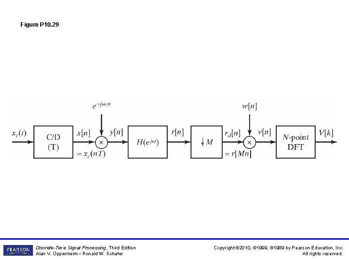
Figure P 10. 29 Discrete-Time Signal Processing, Third Edition Alan V. Oppenheim • Ronald W. Schafer Copyright © 2010, © 1999, © 1989 by Pearson Education, Inc. All rights reserved.

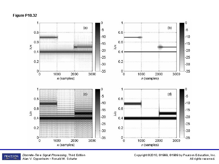
Figure P 10. 32 Discrete-Time Signal Processing, Third Edition Alan V. Oppenheim • Ronald W. Schafer Copyright © 2010, © 1999, © 1989 by Pearson Education, Inc. All rights reserved.

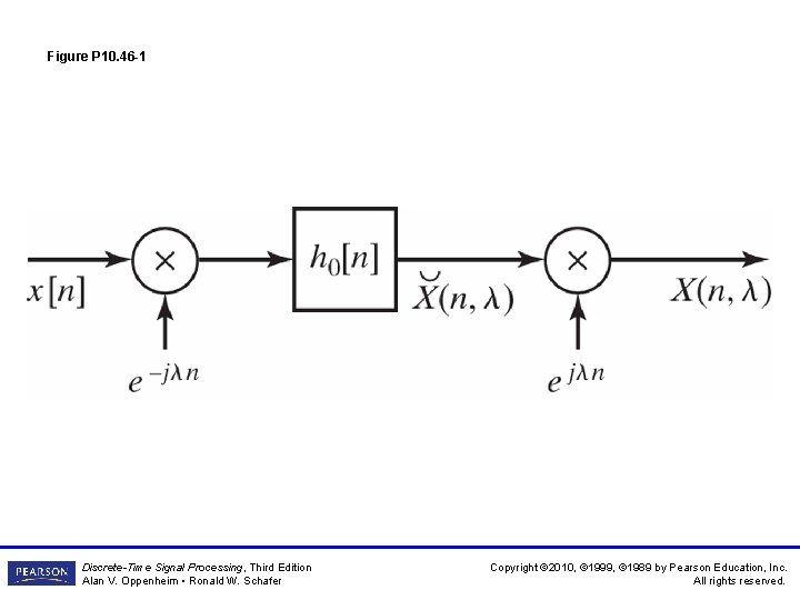
Figure P 10. 46 -1 Discrete-Time Signal Processing, Third Edition Alan V. Oppenheim • Ronald W. Schafer Copyright © 2010, © 1999, © 1989 by Pearson Education, Inc. All rights reserved.

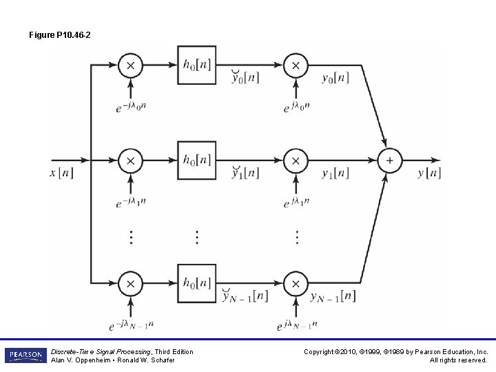
Figure P 10. 46 -2 Discrete-Time Signal Processing, Third Edition Alan V. Oppenheim • Ronald W. Schafer Copyright © 2010, © 1999, © 1989 by Pearson Education, Inc. All rights reserved.

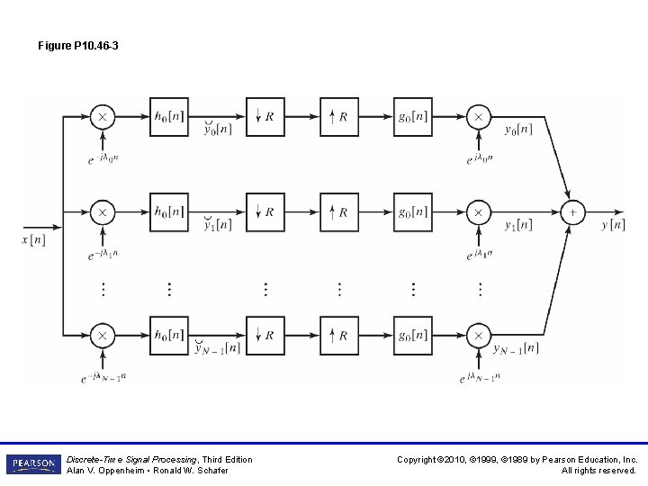
Figure P 10. 46 -3 Discrete-Time Signal Processing, Third Edition Alan V. Oppenheim • Ronald W. Schafer Copyright © 2010, © 1999, © 1989 by Pearson Education, Inc. All rights reserved.

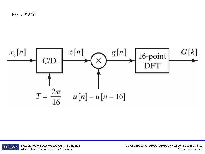
Figure P 10. 48 Discrete-Time Signal Processing, Third Edition Alan V. Oppenheim • Ronald W. Schafer Copyright © 2010, © 1999, © 1989 by Pearson Education, Inc. All rights reserved.

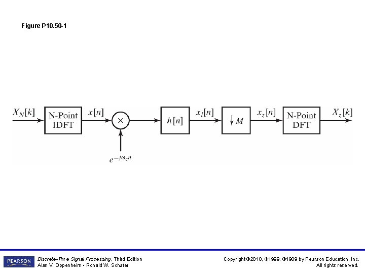
Figure P 10. 50 -1 Discrete-Time Signal Processing, Third Edition Alan V. Oppenheim • Ronald W. Schafer Copyright © 2010, © 1999, © 1989 by Pearson Education, Inc. All rights reserved.

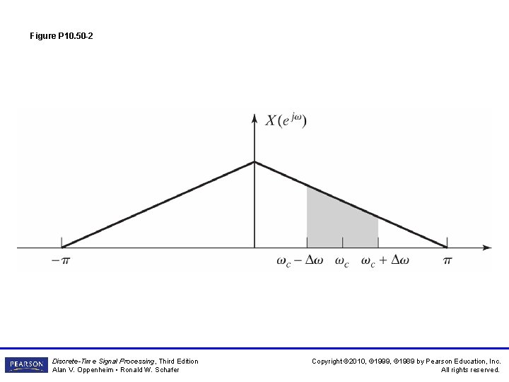
Figure P 10. 50 -2 Discrete-Time Signal Processing, Third Edition Alan V. Oppenheim • Ronald W. Schafer Copyright © 2010, © 1999, © 1989 by Pearson Education, Inc. All rights reserved.

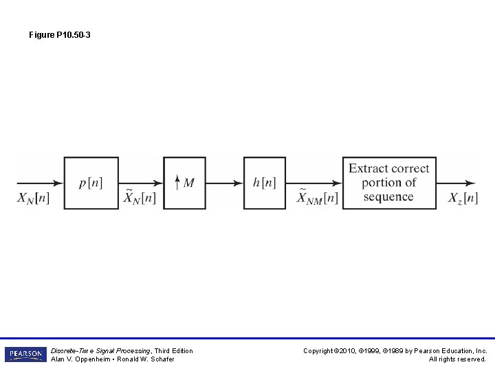
Figure P 10. 50 -3 Discrete-Time Signal Processing, Third Edition Alan V. Oppenheim • Ronald W. Schafer Copyright © 2010, © 1999, © 1989 by Pearson Education, Inc. All rights reserved.