University of Kurdistan Digital Image Processing DIP Lecture
![Bit plane slicing (cont. . ) [10000000] [01000000] [00100000] [00001000] [00000100] [00000001] Digital Image Bit plane slicing (cont. . ) [10000000] [01000000] [00100000] [00001000] [00000100] [00000001] Digital Image](https://slidetodoc.com/presentation_image/bf6a62b28d65a237899d0f85cb776f67/image-48.jpg)
- Slides: 96

University of Kurdistan Digital Image Processing (DIP) Lecture 3: Image Enhancement in the Spatial Domain Instructor: Kaveh Mollazade, Ph. D. Department of Biosystems Engineering, Faculty of Agriculture, University of Kurdistan, Sanandaj, IRAN.

Content • In this lecture, we will look at image enhancement techniques working in the spatial domain: – What is image enhancement? – Different kinds of image enhancement – Histogram processing – Point processing – Neighborhood operations – Spatial filtering operations Digital Image Processing – Department of Biosystems Engineering – University of Kurdistan http: //agri. uok. ac. ir/kmollazade 1

A note about grey levels • So far when we have spoken about image grey level values we have said they are in the range [0, 255]. – Where 0 is black and 255 is white. • There is no reason why we have to use this range. – The range [0, 255] stems from display technologies. • For many of the image processing operations in this lecture, grey levels are assumed to be given in the range [0. 0, 1. 0]. Digital Image Processing – Department of Biosystems Engineering – University of Kurdistan http: //agri. uok. ac. ir/kmollazade 2

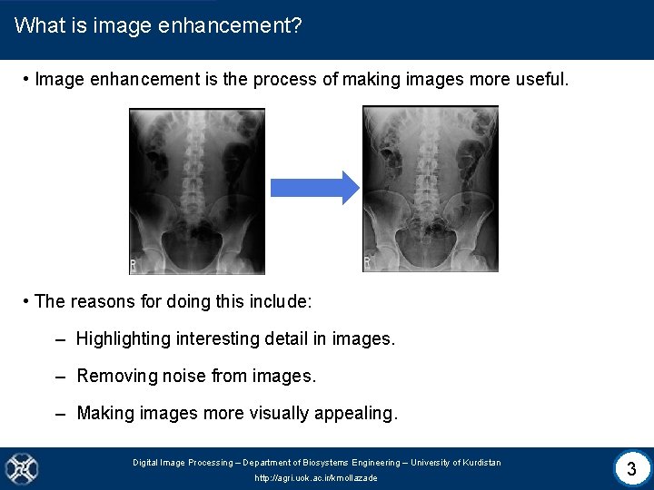
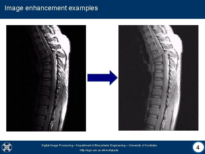
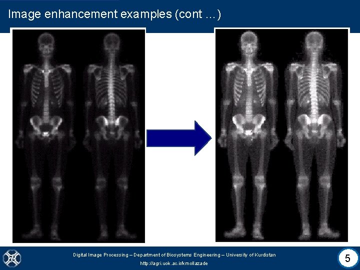
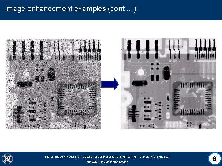
What is image enhancement? • Image enhancement is the process of making images more useful. • The reasons for doing this include: – Highlighting interesting detail in images. – Removing noise from images. – Making images more visually appealing. Digital Image Processing – Department of Biosystems Engineering – University of Kurdistan http: //agri. uok. ac. ir/kmollazade 3

Image enhancement examples Digital Image Processing – Department of Biosystems Engineering – University of Kurdistan http: //agri. uok. ac. ir/kmollazade 4

Image enhancement examples (cont …) Digital Image Processing – Department of Biosystems Engineering – University of Kurdistan http: //agri. uok. ac. ir/kmollazade 5

Image enhancement examples (cont …) Digital Image Processing – Department of Biosystems Engineering – University of Kurdistan http: //agri. uok. ac. ir/kmollazade 6

Spatial & frequency domains • There are two broad categories of image enhancement techniques: 1. Spatial domain techniques: • Direct manipulation of image pixels. 2. Frequency domain techniques: • Manipulation of Fourier transform or wavelet transform of an image. • For the moment we will concentrate on techniques that operate in the spatial domain. Digital Image Processing – Department of Biosystems Engineering – University of Kurdistan http: //agri. uok. ac. ir/kmollazade 7

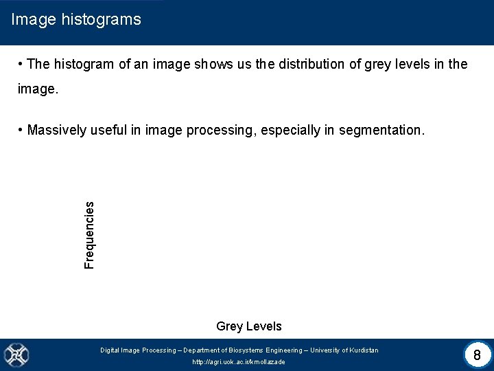
Image histograms • The histogram of an image shows us the distribution of grey levels in the image. Frequencies • Massively useful in image processing, especially in segmentation. Grey Levels Digital Image Processing – Department of Biosystems Engineering – University of Kurdistan http: //agri. uok. ac. ir/kmollazade 8

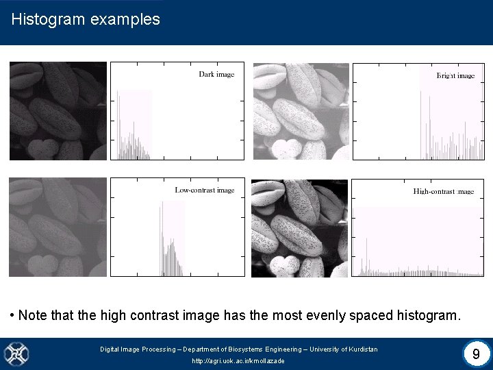
Histogram examples • Note that the high contrast image has the most evenly spaced histogram. Digital Image Processing – Department of Biosystems Engineering – University of Kurdistan http: //agri. uok. ac. ir/kmollazade 9

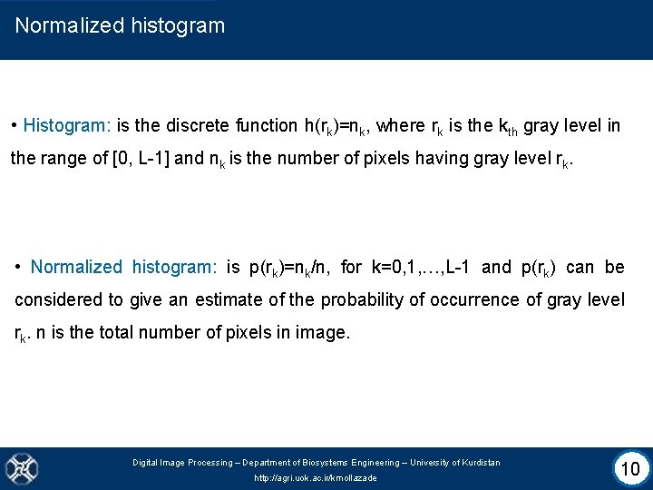
Normalized histogram • Histogram: is the discrete function h(rk)=nk, where rk is the kth gray level in the range of [0, L-1] and nk is the number of pixels having gray level rk. • Normalized histogram: is p(rk)=nk/n, for k=0, 1, …, L-1 and p(rk) can be considered to give an estimate of the probability of occurrence of gray level rk. n is the total number of pixels in image. Digital Image Processing – Department of Biosystems Engineering – University of Kurdistan http: //agri. uok. ac. ir/kmollazade 10

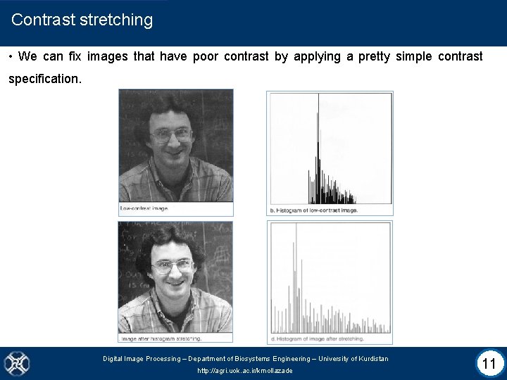
Contrast stretching • We can fix images that have poor contrast by applying a pretty simple contrast specification. Digital Image Processing – Department of Biosystems Engineering – University of Kurdistan http: //agri. uok. ac. ir/kmollazade 11

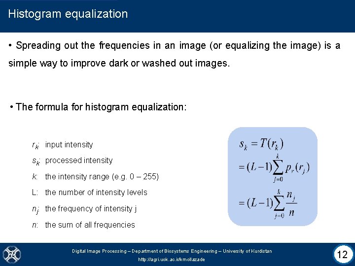
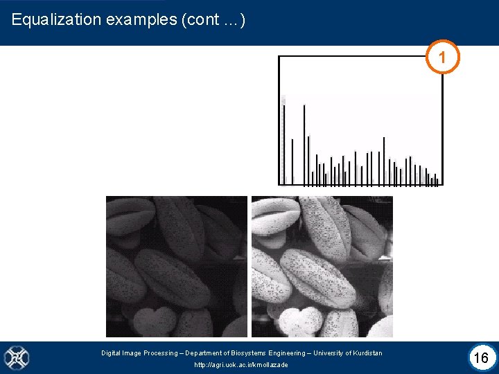
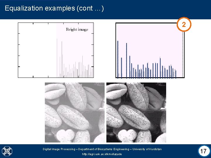
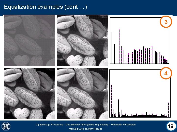
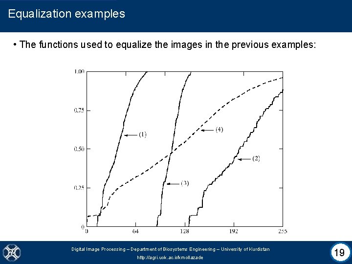
Histogram equalization • Spreading out the frequencies in an image (or equalizing the image) is a simple way to improve dark or washed out images. • The formula for histogram equalization: rk: input intensity sk: processed intensity k: the intensity range (e. g. 0 – 255) L: the number of intensity levels nj: the frequency of intensity j n: the sum of all frequencies Digital Image Processing – Department of Biosystems Engineering – University of Kurdistan http: //agri. uok. ac. ir/kmollazade 12

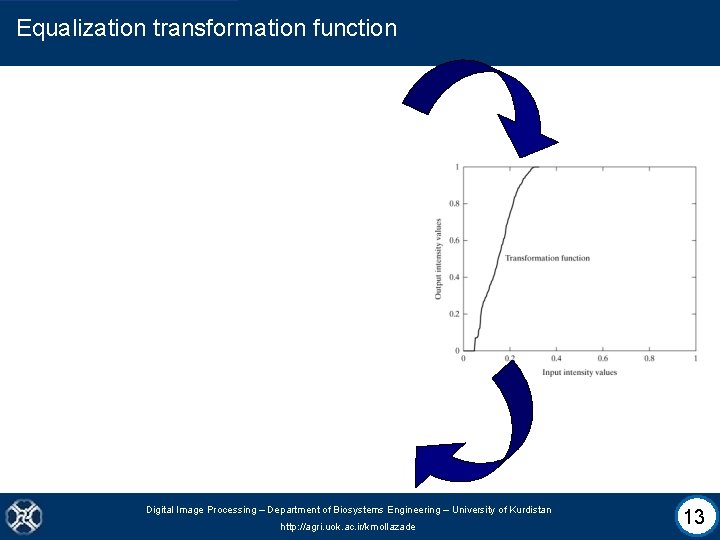
Equalization transformation function Digital Image Processing – Department of Biosystems Engineering – University of Kurdistan http: //agri. uok. ac. ir/kmollazade 13

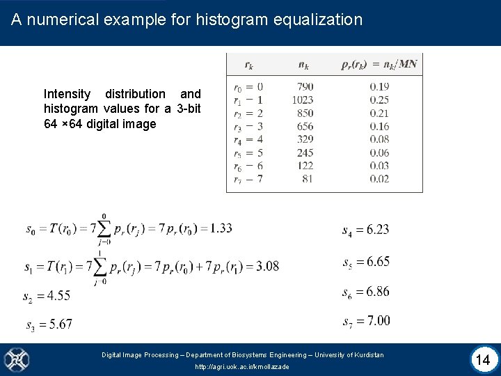
A numerical example for histogram equalization Intensity distribution and histogram values for a 3 -bit 64 × 64 digital image Digital Image Processing – Department of Biosystems Engineering – University of Kurdistan http: //agri. uok. ac. ir/kmollazade 14

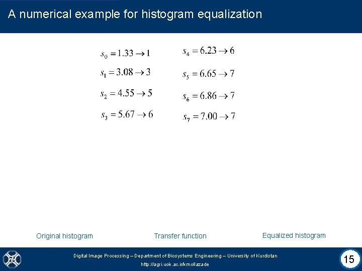
A numerical example for histogram equalization Original histogram Transfer function Equalized histogram Digital Image Processing – Department of Biosystems Engineering – University of Kurdistan http: //agri. uok. ac. ir/kmollazade 15

Equalization examples (cont …) 1 Digital Image Processing – Department of Biosystems Engineering – University of Kurdistan http: //agri. uok. ac. ir/kmollazade 16

Equalization examples (cont …) 2 Digital Image Processing – Department of Biosystems Engineering – University of Kurdistan http: //agri. uok. ac. ir/kmollazade 17

Equalization examples (cont …) 3 4 Digital Image Processing – Department of Biosystems Engineering – University of Kurdistan http: //agri. uok. ac. ir/kmollazade 18

Equalization examples • The functions used to equalize the images in the previous examples: Digital Image Processing – Department of Biosystems Engineering – University of Kurdistan http: //agri. uok. ac. ir/kmollazade 19

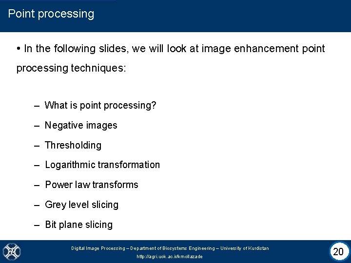
Point processing • In the following slides, we will look at image enhancement point processing techniques: – What is point processing? – Negative images – Thresholding – Logarithmic transformation – Power law transforms – Grey level slicing – Bit plane slicing Digital Image Processing – Department of Biosystems Engineering – University of Kurdistan http: //agri. uok. ac. ir/kmollazade 20

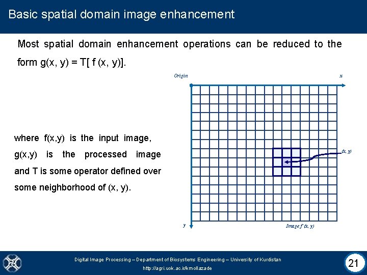
Basic spatial domain image enhancement Most spatial domain enhancement operations can be reduced to the form g(x, y) = T[ f (x, y)]. Origin x where f(x, y) is the input image, g(x, y) is the processed (x, y) image and T is some operator defined over some neighborhood of (x, y). y Digital Image Processing – Department of Biosystems Engineering – University of Kurdistan http: //agri. uok. ac. ir/kmollazade Image f (x, y) 21

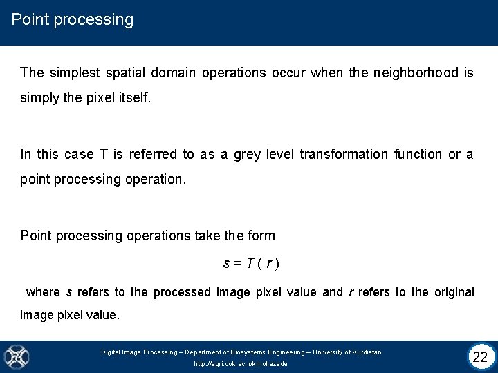
Point processing The simplest spatial domain operations occur when the neighborhood is simply the pixel itself. In this case T is referred to as a grey level transformation function or a point processing operation. Point processing operations take the form s=T(r) where s refers to the processed image pixel value and r refers to the original image pixel value. Digital Image Processing – Department of Biosystems Engineering – University of Kurdistan http: //agri. uok. ac. ir/kmollazade 22

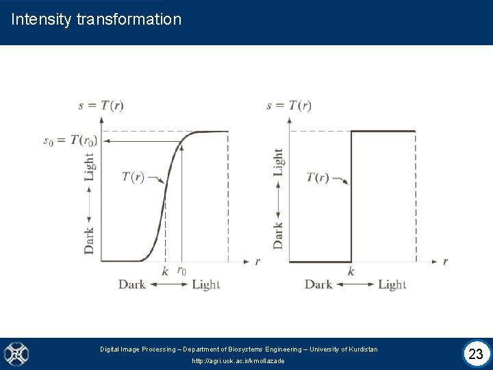
Intensity transformation Digital Image Processing – Department of Biosystems Engineering – University of Kurdistan http: //agri. uok. ac. ir/kmollazade 23

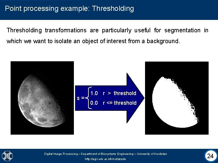
Point processing example: Thresholding transformations are particularly useful for segmentation in which we want to isolate an object of interest from a background. s= 1. 0 r > threshold 0. 0 r <= threshold Digital Image Processing – Department of Biosystems Engineering – University of Kurdistan http: //agri. uok. ac. ir/kmollazade 24

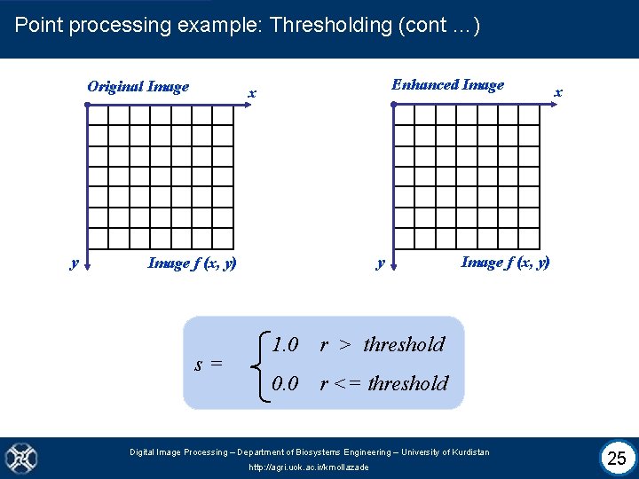
Point processing example: Thresholding (cont …) Original Image y Enhanced Image x y Image f (x, y) s= 1. 0 r > threshold 0. 0 r <= threshold Image f (x, y) Digital Image Processing – Department of Biosystems Engineering – University of Kurdistan http: //agri. uok. ac. ir/kmollazade x 25

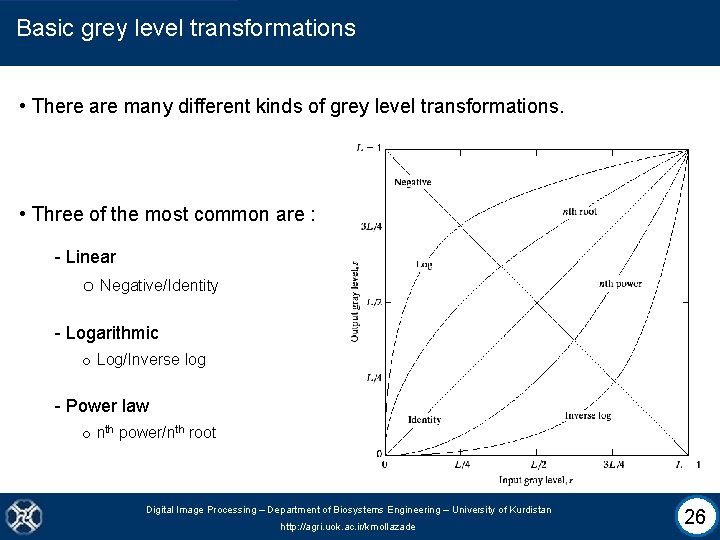
Basic grey level transformations • There are many different kinds of grey level transformations. • Three of the most common are : - Linear o Negative/Identity - Logarithmic o Log/Inverse log - Power law o nth power/nth root Digital Image Processing – Department of Biosystems Engineering – University of Kurdistan http: //agri. uok. ac. ir/kmollazade 26

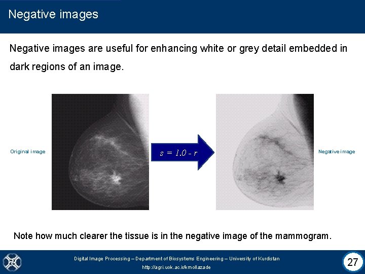
Negative images are useful for enhancing white or grey detail embedded in dark regions of an image. Original image s = 1. 0 - r Negative image Note how much clearer the tissue is in the negative image of the mammogram. Digital Image Processing – Department of Biosystems Engineering – University of Kurdistan http: //agri. uok. ac. ir/kmollazade 27

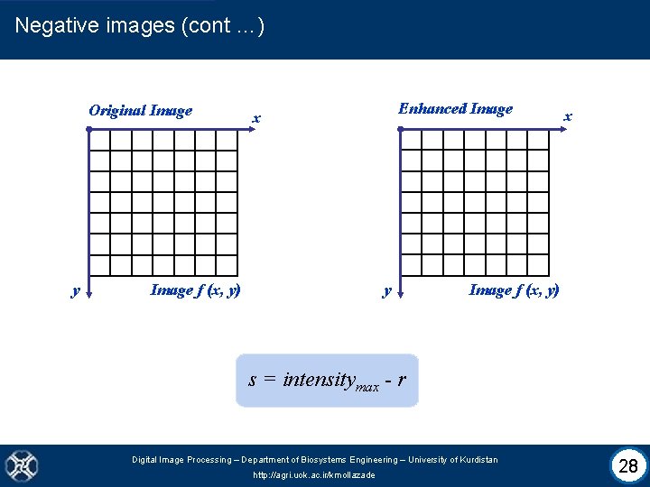
Negative images (cont …) Original Image y Enhanced Image x y Image f (x, y) x Image f (x, y) s = intensitymax - r Digital Image Processing – Department of Biosystems Engineering – University of Kurdistan http: //agri. uok. ac. ir/kmollazade 28

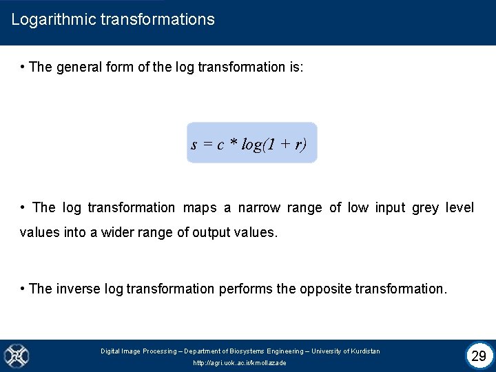
Logarithmic transformations • The general form of the log transformation is: s = c * log(1 + r) • The log transformation maps a narrow range of low input grey level values into a wider range of output values. • The inverse log transformation performs the opposite transformation. Digital Image Processing – Department of Biosystems Engineering – University of Kurdistan http: //agri. uok. ac. ir/kmollazade 29

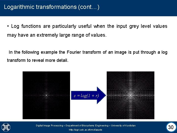
Logarithmic transformations (cont…) • Log functions are particularly useful when the input grey level values may have an extremely large range of values. In the following example the Fourier transform of an image is put through a log transform to reveal more detail. s = log(1 + r) Digital Image Processing – Department of Biosystems Engineering – University of Kurdistan http: //agri. uok. ac. ir/kmollazade 30

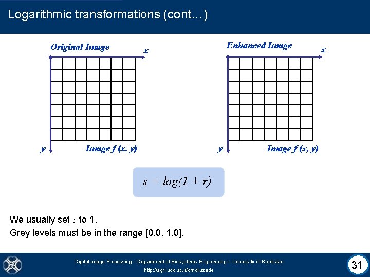
Logarithmic transformations (cont…) Original Image y Enhanced Image x y Image f (x, y) x Image f (x, y) s = log(1 + r) We usually set c to 1. Grey levels must be in the range [0. 0, 1. 0]. Digital Image Processing – Department of Biosystems Engineering – University of Kurdistan http: //agri. uok. ac. ir/kmollazade 31

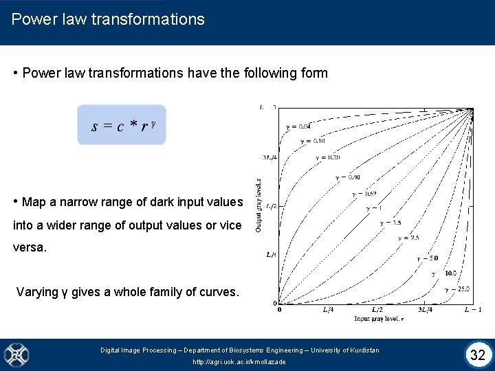
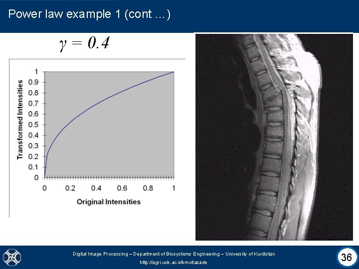
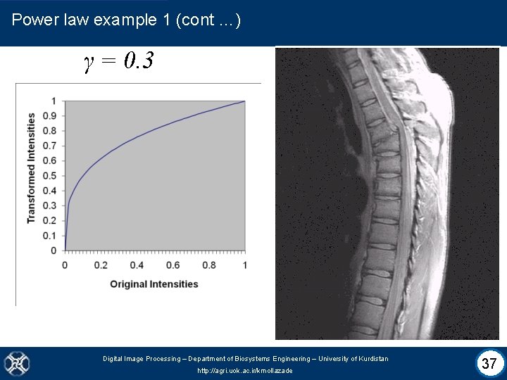
Power law transformations • Power law transformations have the following form s=c*rγ • Map a narrow range of dark input values into a wider range of output values or vice versa. Varying γ gives a whole family of curves. Digital Image Processing – Department of Biosystems Engineering – University of Kurdistan http: //agri. uok. ac. ir/kmollazade 32

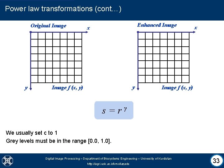
Power law transformations (cont…) Original Image y Enhanced Image x y Image f (x, y) x Image f (x, y) s=rγ We usually set c to 1 Grey levels must be in the range [0. 0, 1. 0]. Digital Image Processing – Department of Biosystems Engineering – University of Kurdistan http: //agri. uok. ac. ir/kmollazade 33

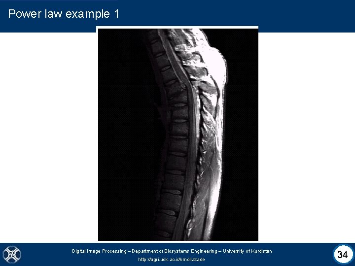
Power law example 1 Digital Image Processing – Department of Biosystems Engineering – University of Kurdistan http: //agri. uok. ac. ir/kmollazade 34

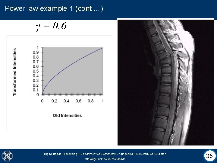
Power law example 1 (cont …) γ = 0. 6 Digital Image Processing – Department of Biosystems Engineering – University of Kurdistan http: //agri. uok. ac. ir/kmollazade 35

Power law example 1 (cont …) γ = 0. 4 Digital Image Processing – Department of Biosystems Engineering – University of Kurdistan http: //agri. uok. ac. ir/kmollazade 36

Power law example 1 (cont …) γ = 0. 3 Digital Image Processing – Department of Biosystems Engineering – University of Kurdistan http: //agri. uok. ac. ir/kmollazade 37

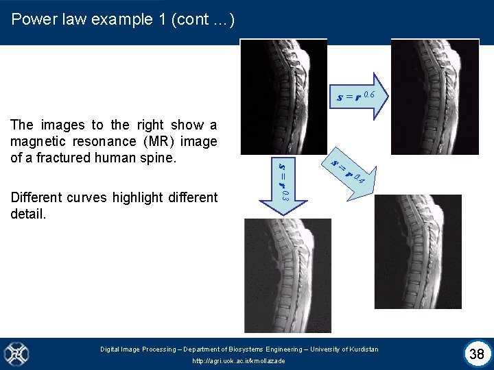
Power law example 1 (cont …) s = r 0. 6 Different curves highlight different detail. s = r 0. 3 The images to the right show a magnetic resonance (MR) image of a fractured human spine. s= r 0. 4 Digital Image Processing – Department of Biosystems Engineering – University of Kurdistan http: //agri. uok. ac. ir/kmollazade 38

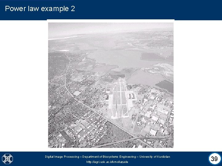
Power law example 2 Digital Image Processing – Department of Biosystems Engineering – University of Kurdistan http: //agri. uok. ac. ir/kmollazade 39

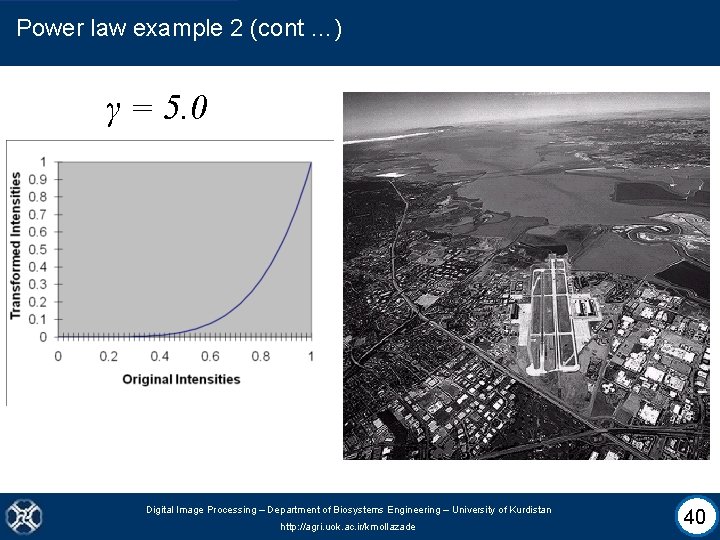
Power law example 2 (cont …) γ = 5. 0 Digital Image Processing – Department of Biosystems Engineering – University of Kurdistan http: //agri. uok. ac. ir/kmollazade 40

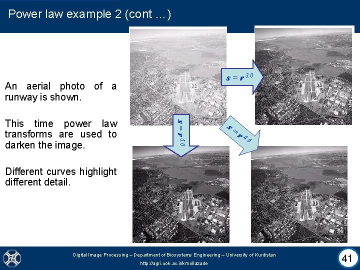
Power law example 2 (cont …) s = r 3. 0 An aerial photo of a runway is shown. s = r 5. 0 This time power law transforms are used to darken the image. s= r 4. 0 Different curves highlight different detail. Digital Image Processing – Department of Biosystems Engineering – University of Kurdistan http: //agri. uok. ac. ir/kmollazade 41

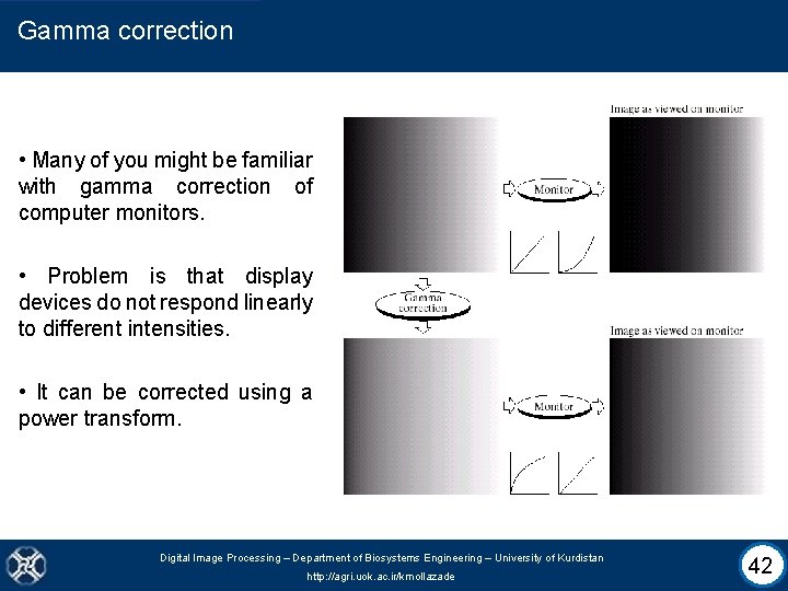
Gamma correction • Many of you might be familiar with gamma correction of computer monitors. • Problem is that display devices do not respond linearly to different intensities. • It can be corrected using a power transform. Digital Image Processing – Department of Biosystems Engineering – University of Kurdistan http: //agri. uok. ac. ir/kmollazade 42

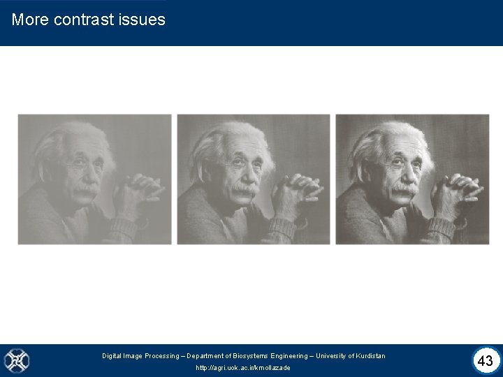
More contrast issues Digital Image Processing – Department of Biosystems Engineering – University of Kurdistan http: //agri. uok. ac. ir/kmollazade 43

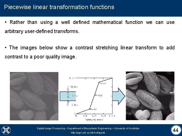
Piecewise linear transformation functions • Rather than using a well defined mathematical function we can use arbitrary user-defined transforms. • The images below show a contrast stretching linear transform to add contrast to a poor quality image. Digital Image Processing – Department of Biosystems Engineering – University of Kurdistan http: //agri. uok. ac. ir/kmollazade 44

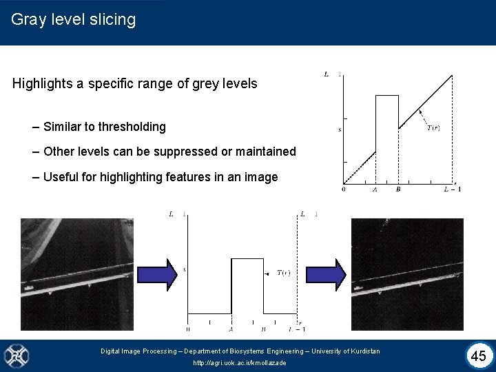
Gray level slicing Highlights a specific range of grey levels – Similar to thresholding – Other levels can be suppressed or maintained – Useful for highlighting features in an image Digital Image Processing – Department of Biosystems Engineering – University of Kurdistan http: //agri. uok. ac. ir/kmollazade 45

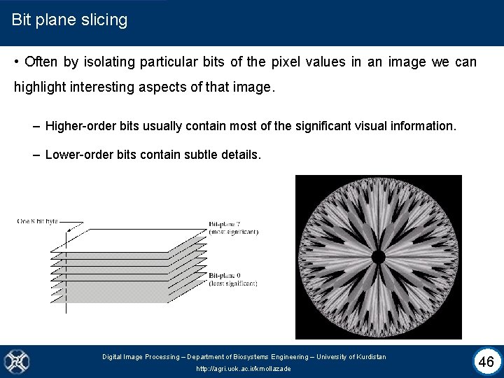
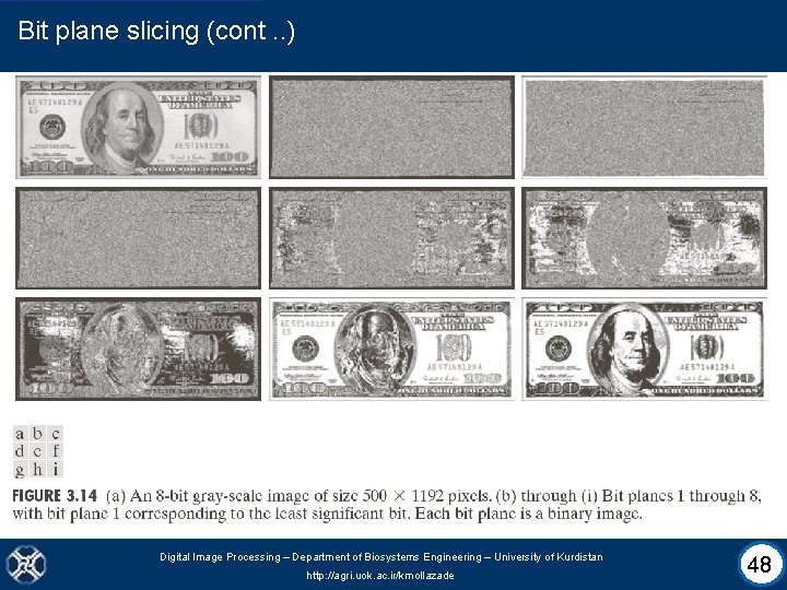
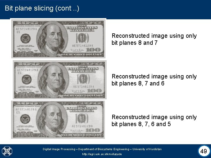
Bit plane slicing • Often by isolating particular bits of the pixel values in an image we can highlight interesting aspects of that image. – Higher-order bits usually contain most of the significant visual information. – Lower-order bits contain subtle details. Digital Image Processing – Department of Biosystems Engineering – University of Kurdistan http: //agri. uok. ac. ir/kmollazade 46
![Bit plane slicing cont 10000000 01000000 00100000 00001000 00000100 00000001 Digital Image Bit plane slicing (cont. . ) [10000000] [01000000] [00100000] [00001000] [00000100] [00000001] Digital Image](https://slidetodoc.com/presentation_image/bf6a62b28d65a237899d0f85cb776f67/image-48.jpg)
Bit plane slicing (cont. . ) [10000000] [01000000] [00100000] [00001000] [00000100] [00000001] Digital Image Processing – Department of Biosystems Engineering – University of Kurdistan http: //agri. uok. ac. ir/kmollazade 47

Bit plane slicing (cont. . ) Digital Image Processing – Department of Biosystems Engineering – University of Kurdistan http: //agri. uok. ac. ir/kmollazade 48

Bit plane slicing (cont. . ) Reconstructed image using only bit planes 8 and 7 Reconstructed image using only bit planes 8, 7 and 6 Reconstructed image using only bit planes 8, 7, 6 and 5 Digital Image Processing – Department of Biosystems Engineering – University of Kurdistan http: //agri. uok. ac. ir/kmollazade 49

Spatial filtering • In the following slides, will look at spatial filtering techniques: – Neighbourhood operations – What is spatial filtering? – Smoothing operations – What happens at the edges? – Correlation and convolution – Sharpening filters (1 st derivative filters and 2 nd derivative filters) – Combining filtering techniques Digital Image Processing – Department of Biosystems Engineering – University of Kurdistan http: //agri. uok. ac. ir/kmollazade 50

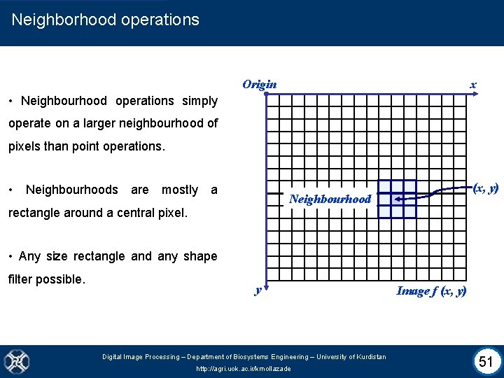
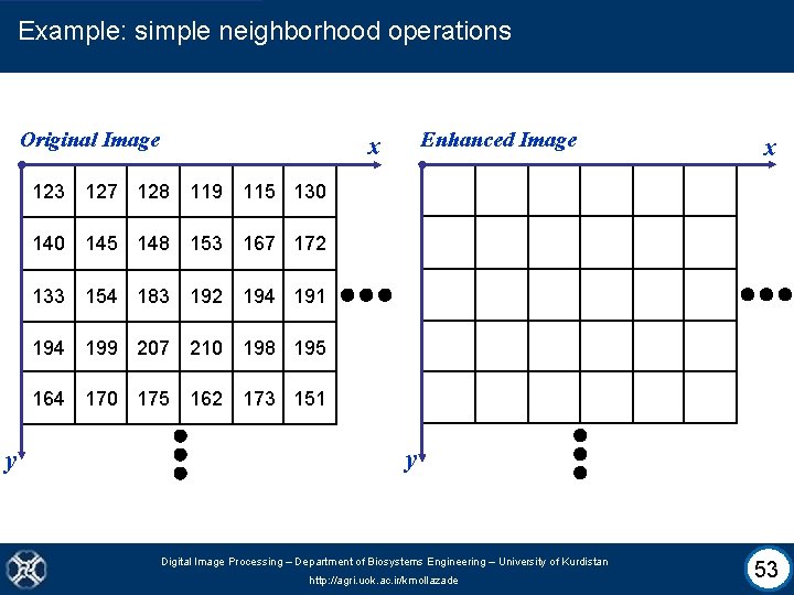
Neighborhood operations Origin x • Neighbourhood operations simply operate on a larger neighbourhood of pixels than point operations. • Neighbourhoods are mostly a (x, y) Neighbourhood rectangle around a central pixel. • Any size rectangle and any shape filter possible. y Digital Image Processing – Department of Biosystems Engineering – University of Kurdistan http: //agri. uok. ac. ir/kmollazade Image f (x, y) 51

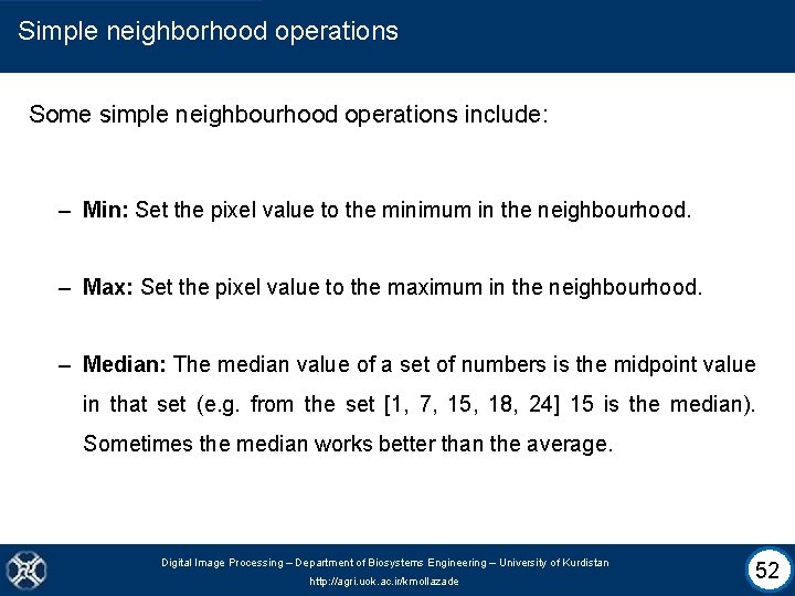
Simple neighborhood operations Some simple neighbourhood operations include: – Min: Set the pixel value to the minimum in the neighbourhood. – Max: Set the pixel value to the maximum in the neighbourhood. – Median: The median value of a set of numbers is the midpoint value in that set (e. g. from the set [1, 7, 15, 18, 24] 15 is the median). Sometimes the median works better than the average. Digital Image Processing – Department of Biosystems Engineering – University of Kurdistan http: //agri. uok. ac. ir/kmollazade 52

Example: simple neighborhood operations Original Image Enhanced Image x x 123 127 128 119 115 130 145 148 153 167 172 133 154 183 192 194 191 194 199 207 210 198 195 164 170 175 162 173 151 y y Digital Image Processing – Department of Biosystems Engineering – University of Kurdistan http: //agri. uok. ac. ir/kmollazade 53

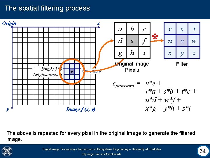
The spatial filtering process Origin x Simple 3*3 Neighbourhood y e 3*3 Filter Image f (x, y) a b c d e f g h i * Original Image Pixels r s t u v w x y z Filter eprocessed = v*e + r*a + s*b + t*c + u*d + w*f + x*g + y*h + z*i The above is repeated for every pixel in the original image to generate the filtered image. Digital Image Processing – Department of Biosystems Engineering – University of Kurdistan http: //agri. uok. ac. ir/kmollazade 54

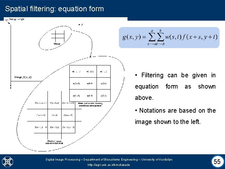
Spatial filtering: equation form • Filtering can be given in equation form as shown above. • Notations are based on the image shown to the left. Digital Image Processing – Department of Biosystems Engineering – University of Kurdistan http: //agri. uok. ac. ir/kmollazade 55

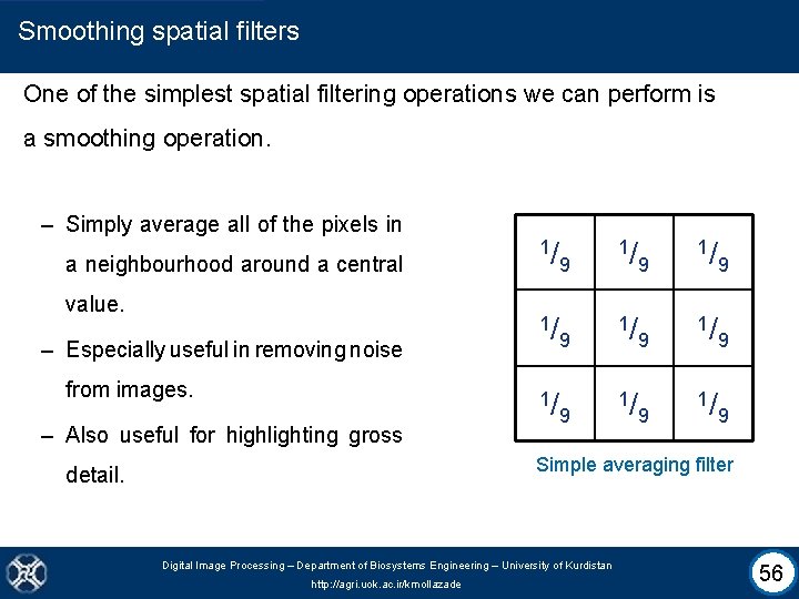
Smoothing spatial filters One of the simplest spatial filtering operations we can perform is a smoothing operation. – Simply average all of the pixels in a neighbourhood around a central value. – Especially useful in removing noise from images. 1/ 1/ 1/ – Also useful for highlighting gross 9 1/ 9 9 1/ 9 Simple averaging filter detail. Digital Image Processing – Department of Biosystems Engineering – University of Kurdistan http: //agri. uok. ac. ir/kmollazade 56

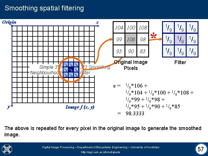
Smoothing spatial filtering Origin x 104 100 108 99 106 98 95 Simple 3*3 Neighbourhood 1/ 100 1/ 108 1/ 104 9 9 9 1/ 99 9 1 106 /9 198 /9 195 /9 190 /9 185 /9 85 Original Image 3*3 Smoothing Pixels 9 1/ 9 1/ 9 Filter e= y 90 * 1/ Image f (x, y) 1/ 9*106 + 1/ *104 + 1/ *100 + 1/ *108 + 9 9 9 1/ *99 + 1/ *98 + 9 9 1/ *95 + 1/ *90 + 1/ *85 9 9 9 = 98. 3333 The above is repeated for every pixel in the original image to generate the smoothed image. Digital Image Processing – Department of Biosystems Engineering – University of Kurdistan http: //agri. uok. ac. ir/kmollazade 57

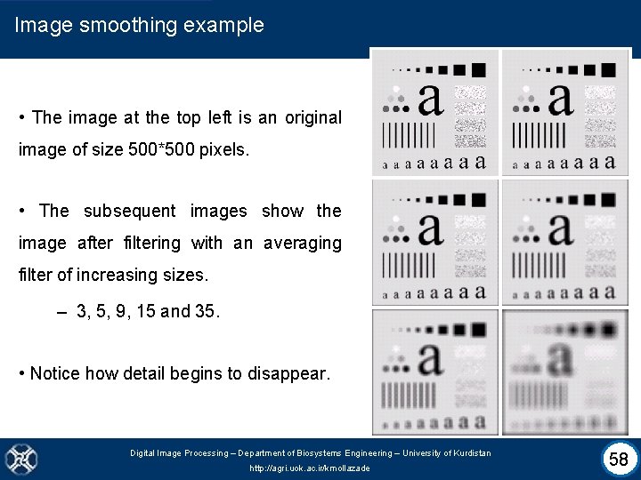
Image smoothing example • The image at the top left is an original image of size 500*500 pixels. • The subsequent images show the image after filtering with an averaging filter of increasing sizes. – 3, 5, 9, 15 and 35. • Notice how detail begins to disappear. Digital Image Processing – Department of Biosystems Engineering – University of Kurdistan http: //agri. uok. ac. ir/kmollazade 58

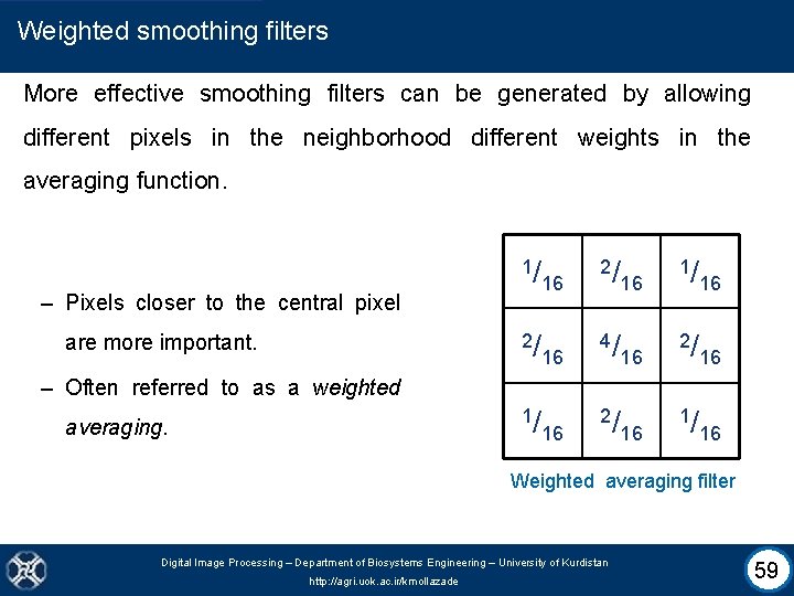
Weighted smoothing filters More effective smoothing filters can be generated by allowing different pixels in the neighborhood different weights in the averaging function. 1/ – Pixels closer to the central pixel 2/ are more important. 16 2/ 16 4/ 16 2/ 16 16 1/ 16 – Often referred to as a weighted 1/ averaging. Weighted averaging filter Digital Image Processing – Department of Biosystems Engineering – University of Kurdistan http: //agri. uok. ac. ir/kmollazade 59

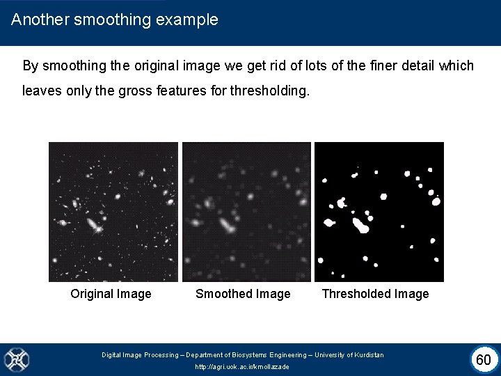
Another smoothing example By smoothing the original image we get rid of lots of the finer detail which leaves only the gross features for thresholding. Original Image Smoothed Image Thresholded Image Digital Image Processing – Department of Biosystems Engineering – University of Kurdistan http: //agri. uok. ac. ir/kmollazade 60

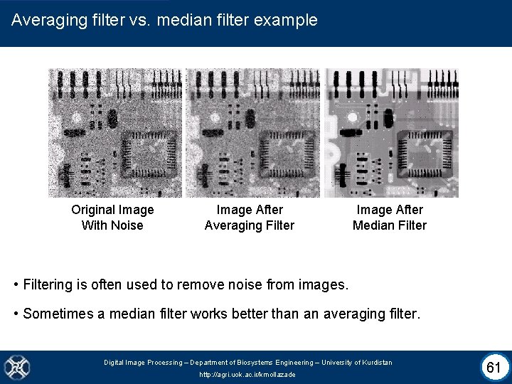
Averaging filter vs. median filter example Original Image With Noise Image After Averaging Filter Image After Median Filter • Filtering is often used to remove noise from images. • Sometimes a median filter works better than an averaging filter. Digital Image Processing – Department of Biosystems Engineering – University of Kurdistan http: //agri. uok. ac. ir/kmollazade 61

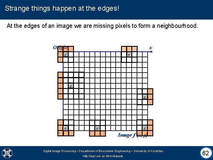
Strange things happen at the edges! At the edges of an image we are missing pixels to form a neighbourhood. Origin x e e e y e e Image f (x, y) Digital Image Processing – Department of Biosystems Engineering – University of Kurdistan http: //agri. uok. ac. ir/kmollazade 62

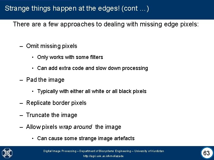
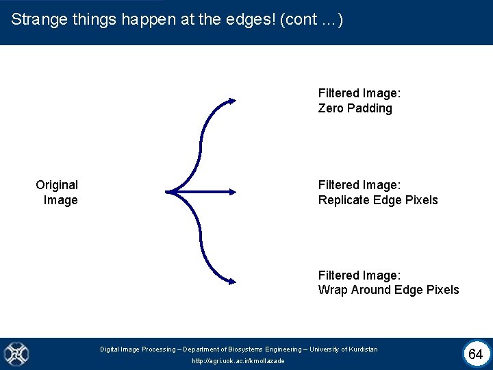
Strange things happen at the edges! (cont …) There a few approaches to dealing with missing edge pixels: – Omit missing pixels • Only works with some filters • Can add extra code and slow down processing – Pad the image • Typically with either all white or all black pixels – Replicate border pixels – Truncate the image – Allow pixels wrap around the image • Can cause some strange image artefacts Digital Image Processing – Department of Biosystems Engineering – University of Kurdistan http: //agri. uok. ac. ir/kmollazade 63

Strange things happen at the edges! (cont …) Filtered Image: Zero Padding Original Image Filtered Image: Replicate Edge Pixels Filtered Image: Wrap Around Edge Pixels Digital Image Processing – Department of Biosystems Engineering – University of Kurdistan http: //agri. uok. ac. ir/kmollazade 64

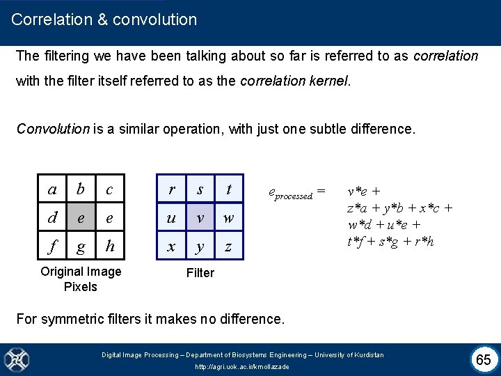
Correlation & convolution The filtering we have been talking about so far is referred to as correlation with the filter itself referred to as the correlation kernel. Convolution is a similar operation, with just one subtle difference. a b c d e e f g h Original Image Pixels * r s t u v w x y z eprocessed = v*e + z*a + y*b + x*c + w*d + u*e + t*f + s*g + r*h Filter For symmetric filters it makes no difference. Digital Image Processing – Department of Biosystems Engineering – University of Kurdistan http: //agri. uok. ac. ir/kmollazade 65

Sharpening spatial filters • Previously we have looked at smoothing filters which remove fine detail. • Sharpening spatial filters seek to highlight fine details: – Remove blurring from images – Highlight edges • Sharpening filters are based on spatial differentiation. Digital Image Processing – Department of Biosystems Engineering – University of Kurdistan http: //agri. uok. ac. ir/kmollazade 66

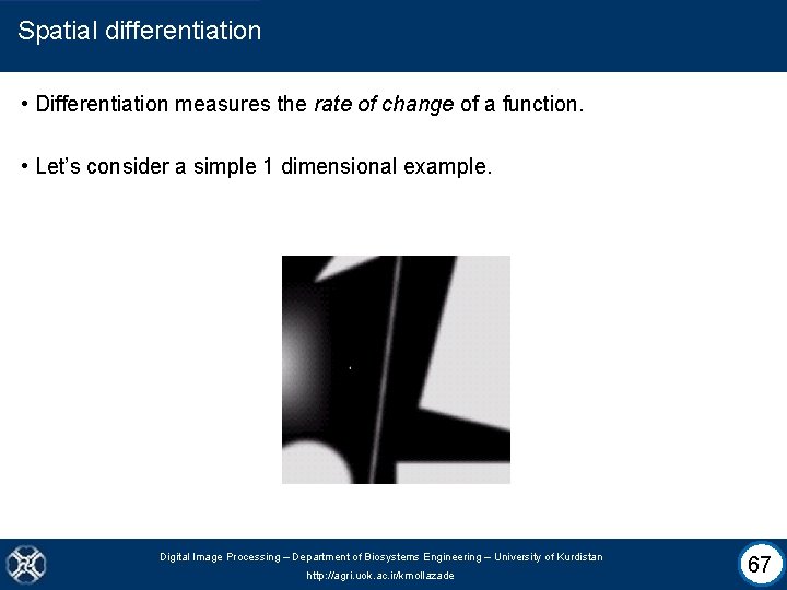
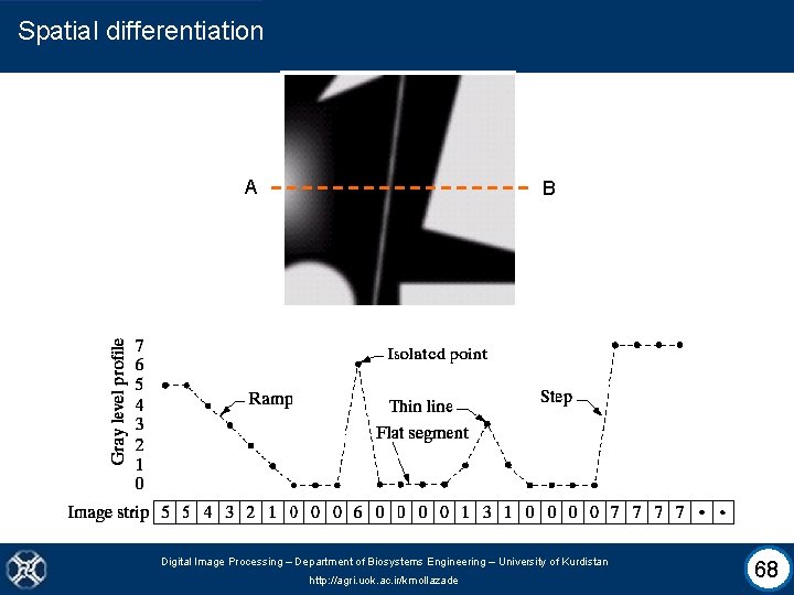
Spatial differentiation • Differentiation measures the rate of change of a function. • Let’s consider a simple 1 dimensional example. Digital Image Processing – Department of Biosystems Engineering – University of Kurdistan http: //agri. uok. ac. ir/kmollazade 67

Spatial differentiation A B Digital Image Processing – Department of Biosystems Engineering – University of Kurdistan http: //agri. uok. ac. ir/kmollazade 68

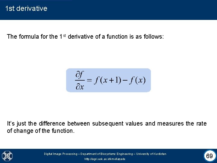
1 st derivative The formula for the 1 st derivative of a function is as follows: It’s just the difference between subsequent values and measures the rate of change of the function. Digital Image Processing – Department of Biosystems Engineering – University of Kurdistan http: //agri. uok. ac. ir/kmollazade 69

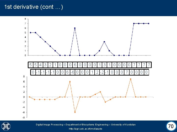
1 st derivative (cont …) 5 5 4 3 2 1 0 0 0 6 0 0 1 3 1 0 0 7 7 0 -1 -1 0 0 6 -6 0 0 0 1 2 -2 -1 0 0 0 7 0 0 Digital Image Processing – Department of Biosystems Engineering – University of Kurdistan http: //agri. uok. ac. ir/kmollazade 70

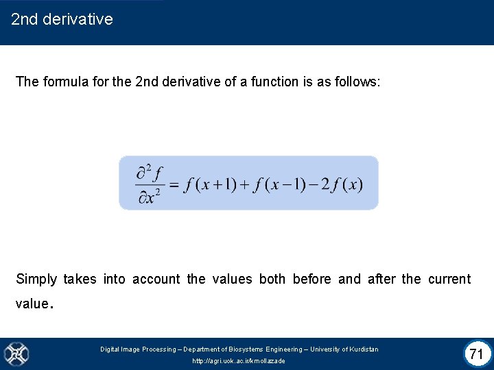
2 nd derivative The formula for the 2 nd derivative of a function is as follows: Simply takes into account the values both before and after the current value . Digital Image Processing – Department of Biosystems Engineering – University of Kurdistan http: //agri. uok. ac. ir/kmollazade 71

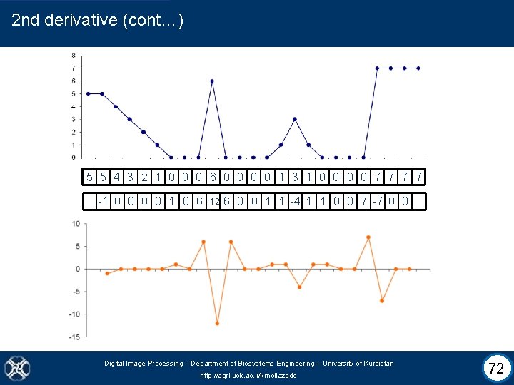
2 nd derivative (cont…) 5 5 4 3 2 1 0 0 0 6 0 0 1 3 1 0 0 7 7 -1 0 0 1 0 6 -12 6 0 0 1 1 -4 1 1 0 0 7 -7 0 0 Digital Image Processing – Department of Biosystems Engineering – University of Kurdistan http: //agri. uok. ac. ir/kmollazade 72

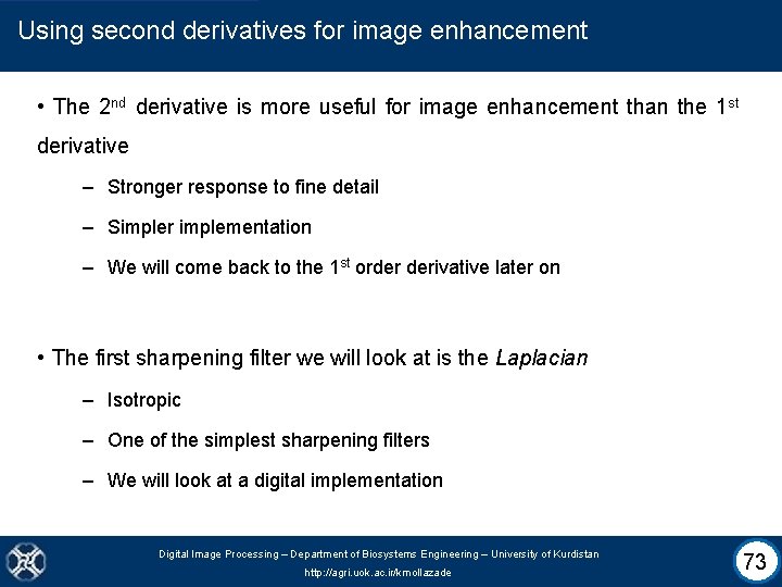
Using second derivatives for image enhancement • The 2 nd derivative is more useful for image enhancement than the 1 st derivative – Stronger response to fine detail – Simpler implementation – We will come back to the 1 st order derivative later on • The first sharpening filter we will look at is the Laplacian – Isotropic – One of the simplest sharpening filters – We will look at a digital implementation Digital Image Processing – Department of Biosystems Engineering – University of Kurdistan http: //agri. uok. ac. ir/kmollazade 73

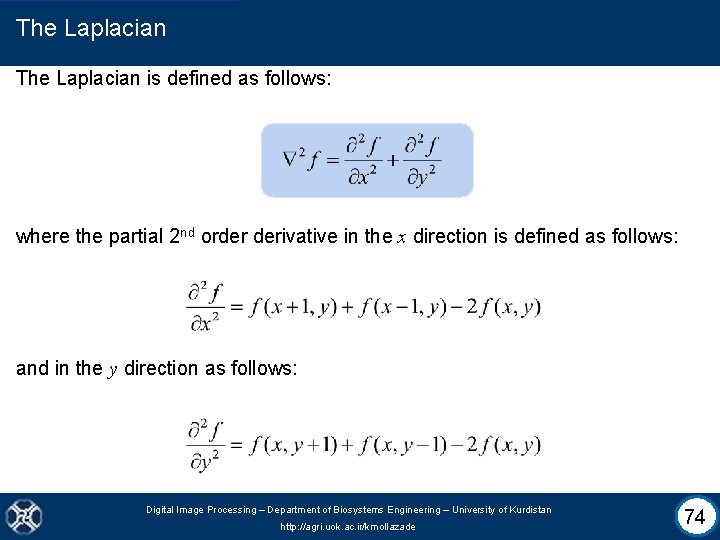
The Laplacian is defined as follows: where the partial 2 nd order derivative in the x direction is defined as follows: and in the y direction as follows: Digital Image Processing – Department of Biosystems Engineering – University of Kurdistan http: //agri. uok. ac. ir/kmollazade 74

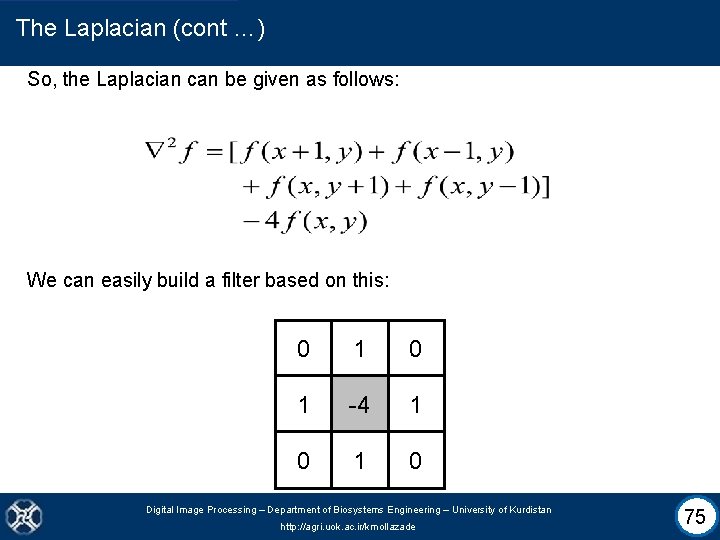
The Laplacian (cont …) So, the Laplacian can be given as follows: We can easily build a filter based on this: 0 1 -4 1 0 Digital Image Processing – Department of Biosystems Engineering – University of Kurdistan http: //agri. uok. ac. ir/kmollazade 75

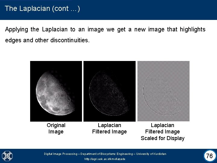
The Laplacian (cont …) Applying the Laplacian to an image we get a new image that highlights edges and other discontinuities. Original Image Laplacian Filtered Image Scaled for Display Digital Image Processing – Department of Biosystems Engineering – University of Kurdistan http: //agri. uok. ac. ir/kmollazade 76

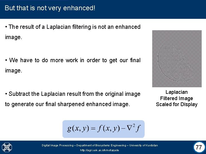
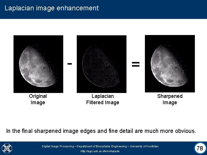
But that is not very enhanced! • The result of a Laplacian filtering is not an enhanced image. • We have to do more work in order to get our final image. • Subtract the Laplacian result from the original image to generate our final sharpened enhanced image. Laplacian Filtered Image Scaled for Display Digital Image Processing – Department of Biosystems Engineering – University of Kurdistan http: //agri. uok. ac. ir/kmollazade 77

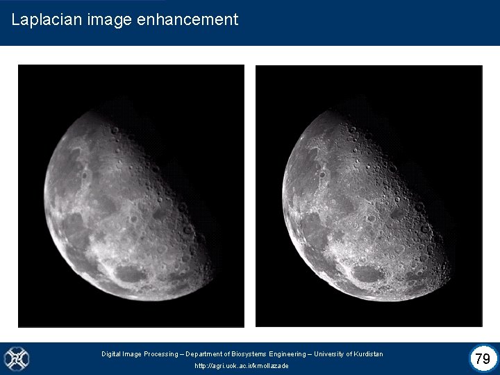
Laplacian image enhancement Original Image = Laplacian Filtered Image Sharpened Image In the final sharpened image edges and fine detail are much more obvious. Digital Image Processing – Department of Biosystems Engineering – University of Kurdistan http: //agri. uok. ac. ir/kmollazade 78

Laplacian image enhancement Digital Image Processing – Department of Biosystems Engineering – University of Kurdistan http: //agri. uok. ac. ir/kmollazade 79

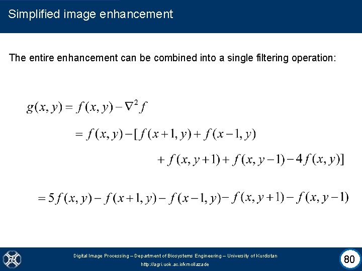
Simplified image enhancement The entire enhancement can be combined into a single filtering operation: Digital Image Processing – Department of Biosystems Engineering – University of Kurdistan http: //agri. uok. ac. ir/kmollazade 80

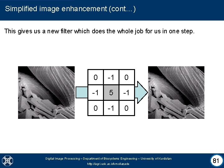
Simplified image enhancement (cont…) This gives us a new filter which does the whole job for us in one step. 0 -1 5 -1 0 Digital Image Processing – Department of Biosystems Engineering – University of Kurdistan http: //agri. uok. ac. ir/kmollazade 81

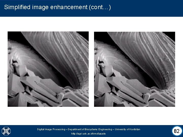
Simplified image enhancement (cont…) Digital Image Processing – Department of Biosystems Engineering – University of Kurdistan http: //agri. uok. ac. ir/kmollazade 82

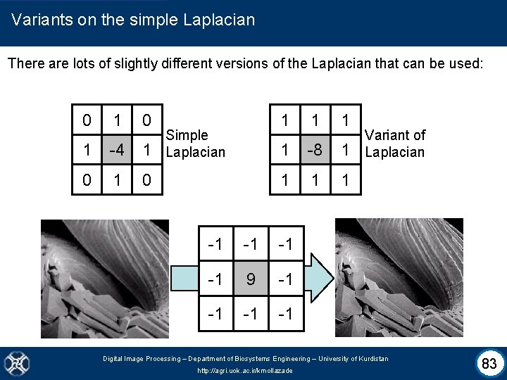
Variants on the simple Laplacian There are lots of slightly different versions of the Laplacian that can be used: 0 1 -4 1 0 Simple Laplacian 1 1 -8 1 1 -1 -1 9 -1 -1 Variant of Laplacian Digital Image Processing – Department of Biosystems Engineering – University of Kurdistan http: //agri. uok. ac. ir/kmollazade 83

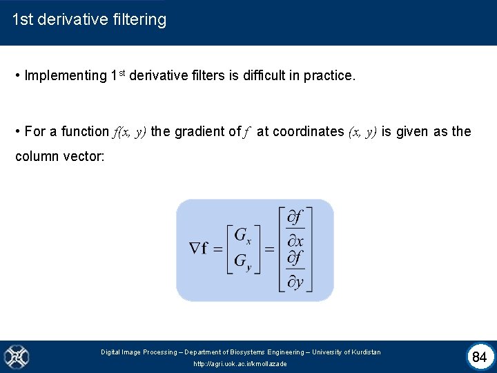
1 st derivative filtering • Implementing 1 st derivative filters is difficult in practice. • For a function f(x, y) the gradient of f at coordinates (x, y) is given as the column vector: Digital Image Processing – Department of Biosystems Engineering – University of Kurdistan http: //agri. uok. ac. ir/kmollazade 84

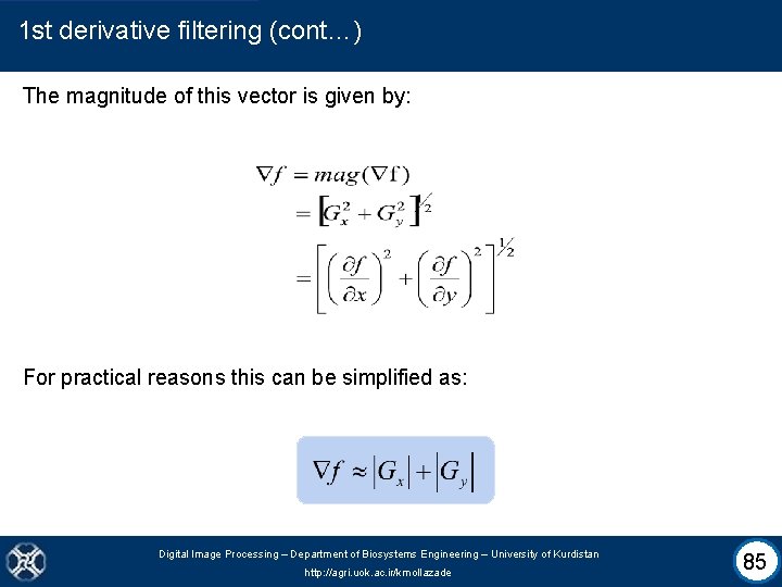
1 st derivative filtering (cont…) The magnitude of this vector is given by: For practical reasons this can be simplified as: Digital Image Processing – Department of Biosystems Engineering – University of Kurdistan http: //agri. uok. ac. ir/kmollazade 85

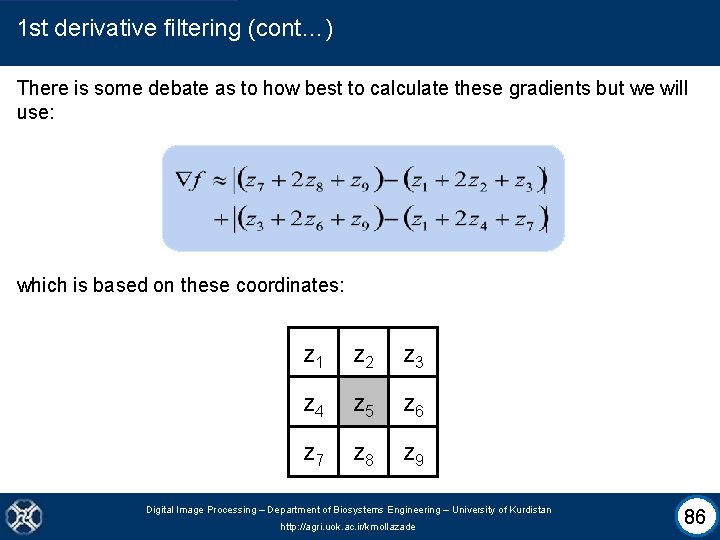
1 st derivative filtering (cont…) There is some debate as to how best to calculate these gradients but we will use: which is based on these coordinates: z 1 z 2 z 3 z 4 z 5 z 6 z 7 z 8 z 9 Digital Image Processing – Department of Biosystems Engineering – University of Kurdistan http: //agri. uok. ac. ir/kmollazade 86

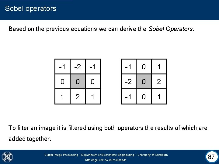
Sobel operators Based on the previous equations we can derive the Sobel Operators. -1 -2 -1 -1 0 0 0 -2 0 2 1 -1 0 1 To filter an image it is filtered using both operators the results of which are added together. Digital Image Processing – Department of Biosystems Engineering – University of Kurdistan http: //agri. uok. ac. ir/kmollazade 87

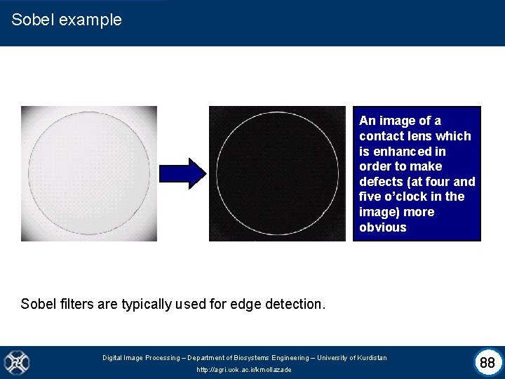
Sobel example An image of a contact lens which is enhanced in order to make defects (at four and five o’clock in the image) more obvious Sobel filters are typically used for edge detection. Digital Image Processing – Department of Biosystems Engineering – University of Kurdistan http: //agri. uok. ac. ir/kmollazade 88

1 st & 2 nd Derivatives Comparing the 1 st and 2 nd derivatives we can conclude the following: – 1 st order derivatives generally produce thicker edges. – 2 nd order derivatives have a stronger response to fine detail e. g. thin lines. – 1 st order derivatives have stronger response to grey level step. – 2 nd order derivatives produce a double response at step changes in grey level. Digital Image Processing – Department of Biosystems Engineering – University of Kurdistan http: //agri. uok. ac. ir/kmollazade 89

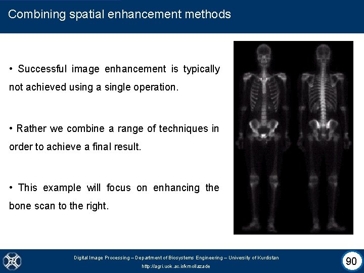
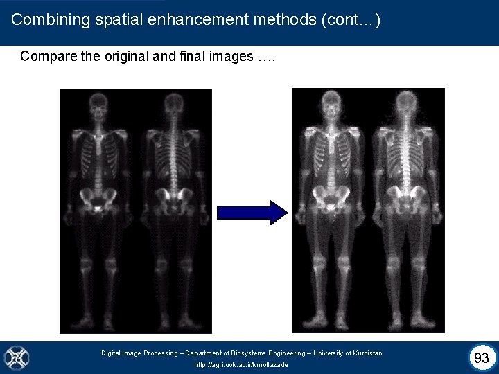
Combining spatial enhancement methods • Successful image enhancement is typically not achieved using a single operation. • Rather we combine a range of techniques in order to achieve a final result. • This example will focus on enhancing the bone scan to the right. Digital Image Processing – Department of Biosystems Engineering – University of Kurdistan http: //agri. uok. ac. ir/kmollazade 90

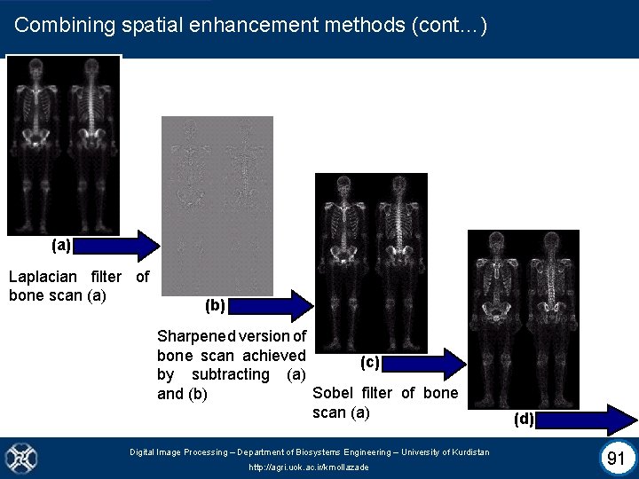
Combining spatial enhancement methods (cont…) (a) Laplacian filter of bone scan (a) (b) Sharpened version of bone scan achieved (c) by subtracting (a) Sobel filter of bone and (b) scan (a) Digital Image Processing – Department of Biosystems Engineering – University of Kurdistan http: //agri. uok. ac. ir/kmollazade (d) 91

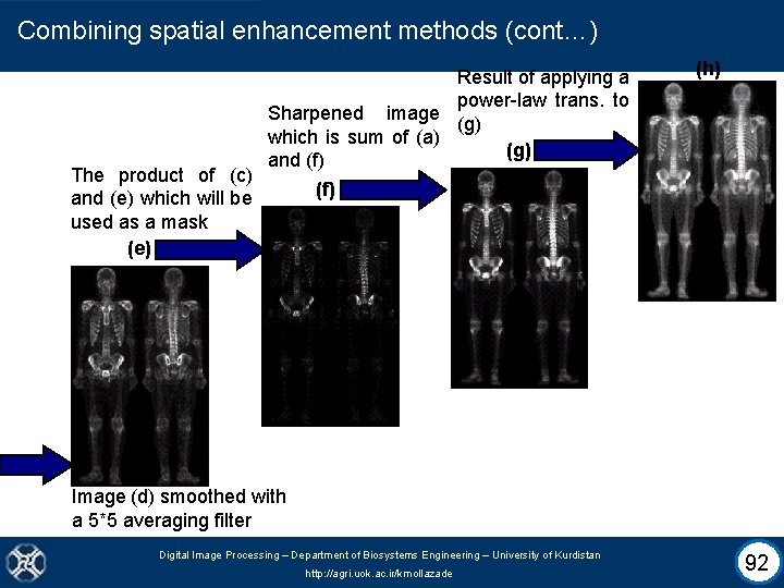
Combining spatial enhancement methods (cont…) The product of (c) and (e) which will be used as a mask (e) Result of applying a power-law trans. to Sharpened image (g) which is sum of (a) (g) and (f) (h) (f) Image (d) smoothed with a 5*5 averaging filter Digital Image Processing – Department of Biosystems Engineering – University of Kurdistan http: //agri. uok. ac. ir/kmollazade 92

Combining spatial enhancement methods (cont…) Compare the original and final images …. Digital Image Processing – Department of Biosystems Engineering – University of Kurdistan http: //agri. uok. ac. ir/kmollazade 93

Summary • We have looked at: – Different kinds of image enhancement – Histograms – Histogram equalisation – Point processing operations – Spatial filtering (Neighbourhood operations, Smoothing filters, Correlation and convolution, Sharpening filters, 1 st derivative filters, 2 nd derivative filters, …). Digital Image Processing – Department of Biosystems Engineering – University of Kurdistan http: //agri. uok. ac. ir/kmollazade 94

Digital Image Processing – Department of Biosystems Engineering – University of Kurdistan http: //agri. uok. ac. ir/kmollazade