Histogram Equalization Continuous Case Idea To find a

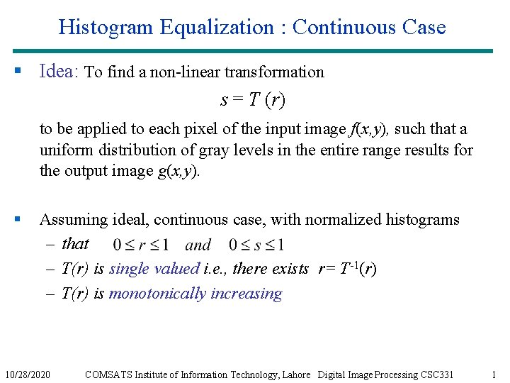
Histogram Equalization : Continuous Case § Idea: To find a non-linear transformation s = T (r) to be applied to each pixel of the input image f(x, y), such that a uniform distribution of gray levels in the entire range results for the output image g(x, y). § Assuming ideal, continuous case, with normalized histograms – that – T(r) is single valued i. e. , there exists r= T-1(r) – T(r) is monotonically increasing 10/28/2020 COMSATS Institute of Information Technology, Lahore Digital Image Processing CSC 331 1

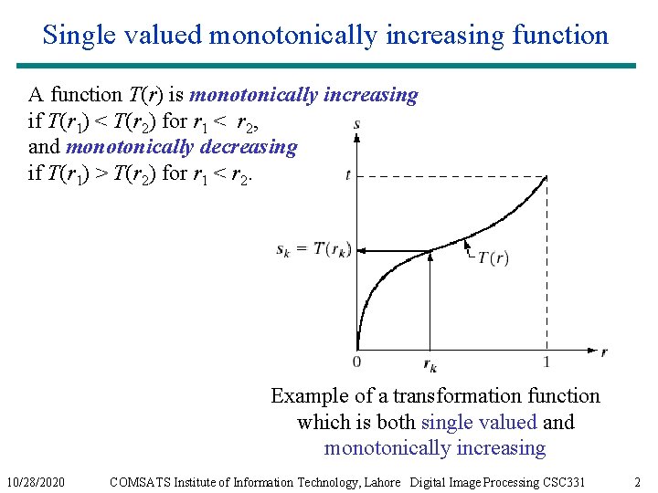
Single valued monotonically increasing function A function T(r) is monotonically increasing if T(r 1) < T(r 2) for r 1 < r 2, and monotonically decreasing if T(r 1) > T(r 2) for r 1 < r 2. Example of a transformation function which is both single valued and monotonically increasing 10/28/2020 COMSATS Institute of Information Technology, Lahore Digital Image Processing CSC 331 2

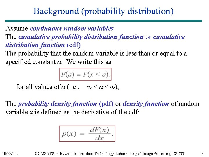
Background (probability distribution) Assume continuous random variables The cumulative probability distribution function or cumulative distribution function (cdf) The probability that the random variable is less than or equal to a specified constant a. We write this as for all values of a (i. e. , < a < ), The probability density function (pdf) or density function of random variable x is defined as the derivative of the cdf: 10/28/2020 COMSATS Institute of Information Technology, Lahore Digital Image Processing CSC 331 3

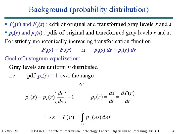
Background (probability distribution) § Fr(r) and Fs(s) : cdfs of original and transformed gray levels r and s. § pr(r) and ps(s) : pdfs of original and transformed gray levels r and s. For strictly monotonically increasing transformation function Fs(s) = Fr(r) or ps(s) ds = pr(r) dr Goal of histogram equalization: Gray levels are uniformly distributed i. e. pdf ps(s) = 1 over the range or 10/28/2020 COMSATS Institute of Information Technology, Lahore Digital Image Processing CSC 331 4

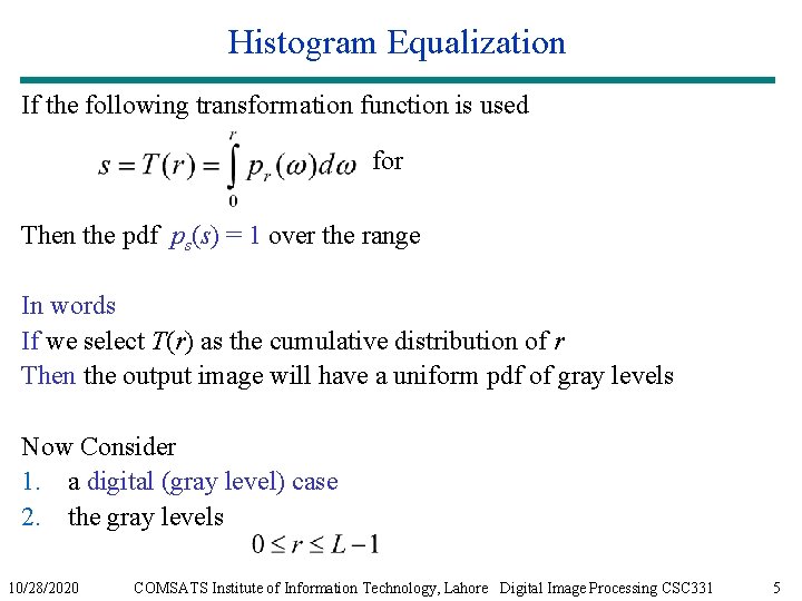
Histogram Equalization If the following transformation function is used for Then the pdf ps(s) = 1 over the range In words If we select T(r) as the cumulative distribution of r Then the output image will have a uniform pdf of gray levels Now Consider 1. a digital (gray level) case 2. the gray levels 10/28/2020 COMSATS Institute of Information Technology, Lahore Digital Image Processing CSC 331 5

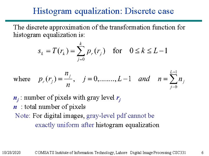
Histogram equalization: Discrete case The discrete approximation of the transformation function for histogram equalization is: where nj : number of pixels with gray level rj n : total number of pixels Note: For digital images, gray-level pdf cannot be exactly uniform after histogram equalization 10/28/2020 COMSATS Institute of Information Technology, Lahore Digital Image Processing CSC 331 6

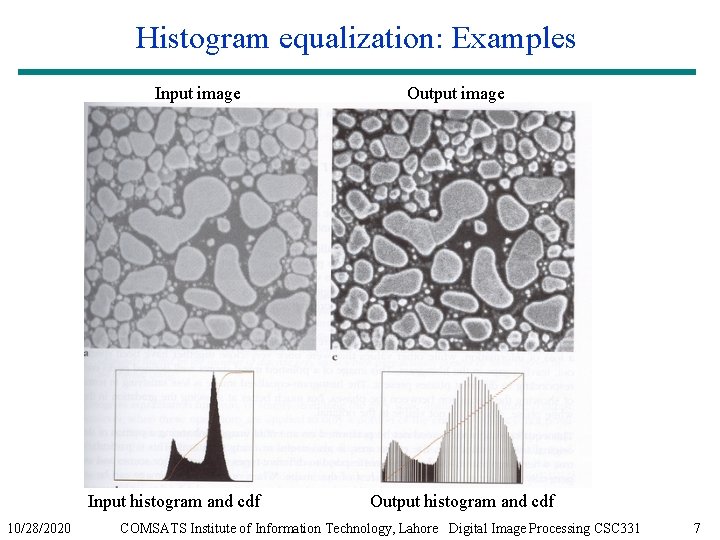
Histogram equalization: Examples Input image Input histogram and cdf 10/28/2020 Output image Output histogram and cdf COMSATS Institute of Information Technology, Lahore Digital Image Processing CSC 331 7

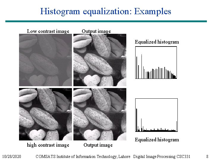
Histogram equalization: Examples Low contrast image Output image Equalized histogram high contrast image 10/28/2020 Output image Equalized histogram COMSATS Institute of Information Technology, Lahore Digital Image Processing CSC 331 8

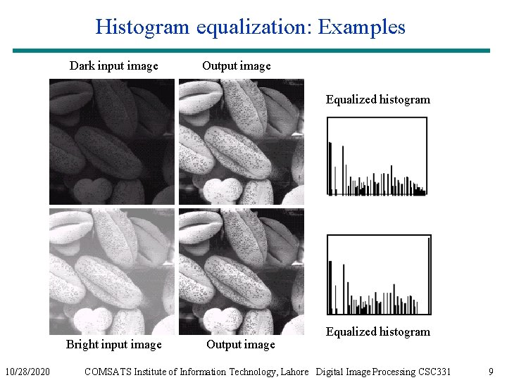
Histogram equalization: Examples Dark input image Output image Equalized histogram Bright input image 10/28/2020 Output image Equalized histogram COMSATS Institute of Information Technology, Lahore Digital Image Processing CSC 331 9

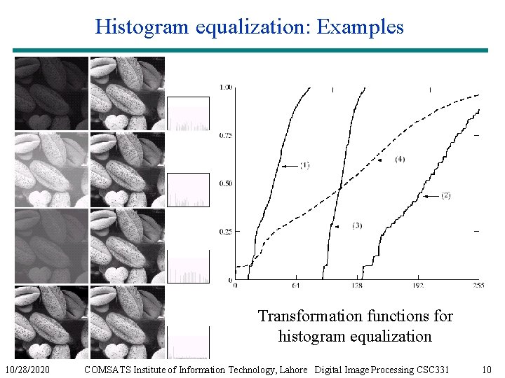
Histogram equalization: Examples Transformation functions for histogram equalization 10/28/2020 COMSATS Institute of Information Technology, Lahore Digital Image Processing CSC 331 10

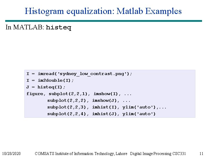
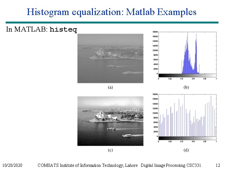
Histogram equalization: Matlab Examples In MATLAB: histeq I = imread('sydney_low_contrast. png'); I = im 2 double(I); J = histeq(I); figure, subplot(2, 2, 1), imshow(I), . . . subplot(2, 2, 2), imshow(J), . . . subplot(2, 2, 3), imhist(I), ylim('auto'), . . . subplot(2, 2, 4), imhist(J), ylim('auto') 10/28/2020 COMSATS Institute of Information Technology, Lahore Digital Image Processing CSC 331 11

Histogram equalization: Matlab Examples In MATLAB: histeq 10/28/2020 COMSATS Institute of Information Technology, Lahore Digital Image Processing CSC 331 12

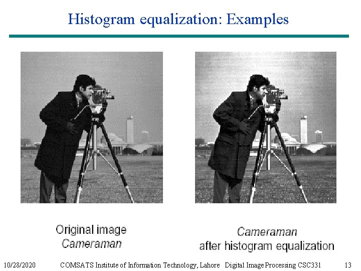
Histogram equalization: Examples 10/28/2020 COMSATS Institute of Information Technology, Lahore Digital Image Processing CSC 331 13

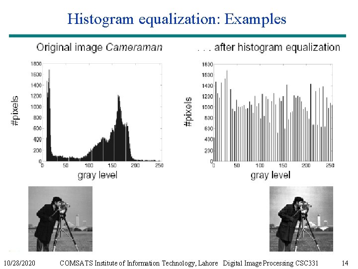
Histogram equalization: Examples 10/28/2020 COMSATS Institute of Information Technology, Lahore Digital Image Processing CSC 331 14

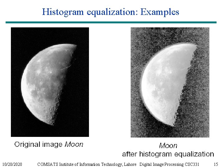
Histogram equalization: Examples 10/28/2020 COMSATS Institute of Information Technology, Lahore Digital Image Processing CSC 331 15

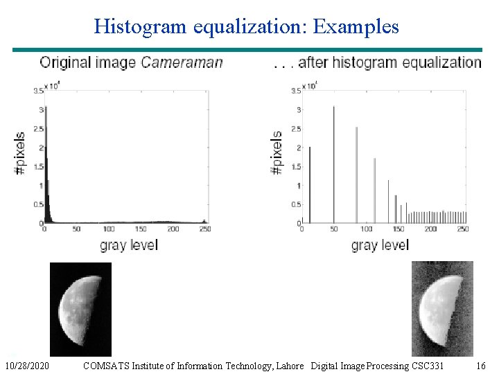
Histogram equalization: Examples 10/28/2020 COMSATS Institute of Information Technology, Lahore Digital Image Processing CSC 331 16

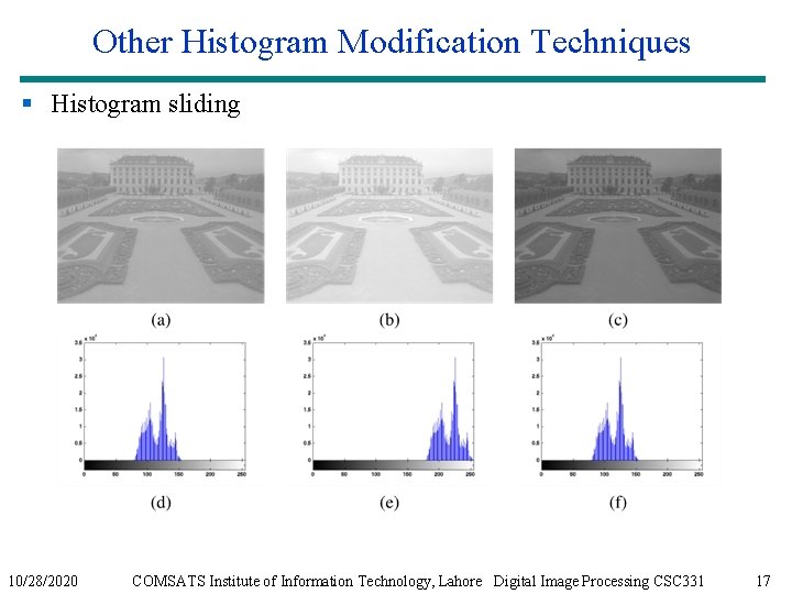
Other Histogram Modification Techniques § Histogram sliding 10/28/2020 COMSATS Institute of Information Technology, Lahore Digital Image Processing CSC 331 17

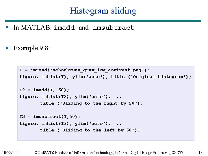
Histogram sliding § In MATLAB: imadd and imsubtract § Example 9. 8: I = imread('schonbrunn_gray_low_contrast. png'); figure, imhist(I), ylim('auto'), title ('Original histogram'); I 2 = imadd(I, 50); figure, imhist(I 2), ylim('auto'), . . . title ('Sliding to the right by 50'); I 3 = imsubtract(I, 50); figure, imhist(I 3), ylim('auto'), . . . title ('Sliding to the left by 50'); 10/28/2020 COMSATS Institute of Information Technology, Lahore Digital Image Processing CSC 331 18

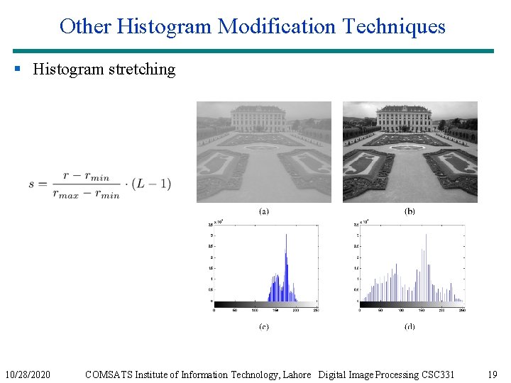
Other Histogram Modification Techniques § Histogram stretching 10/28/2020 COMSATS Institute of Information Technology, Lahore Digital Image Processing CSC 331 19

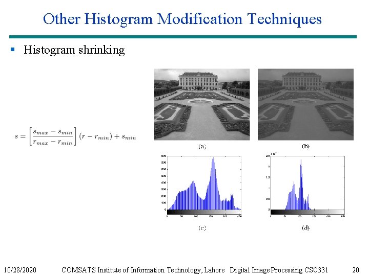
Other Histogram Modification Techniques § Histogram shrinking 10/28/2020 COMSATS Institute of Information Technology, Lahore Digital Image Processing CSC 331 20

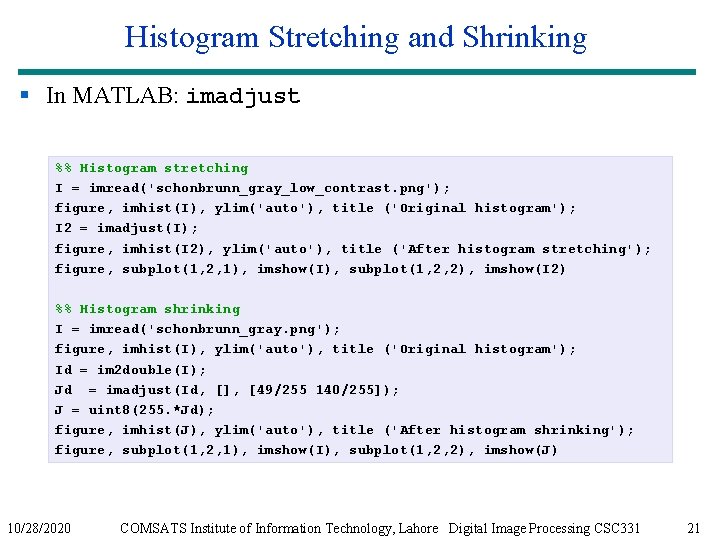
Histogram Stretching and Shrinking § In MATLAB: imadjust %% Histogram stretching I = imread('schonbrunn_gray_low_contrast. png'); figure, imhist(I), ylim('auto'), title ('Original histogram'); I 2 = imadjust(I); figure, imhist(I 2), ylim('auto'), title ('After histogram stretching'); figure, subplot(1, 2, 1), imshow(I), subplot(1, 2, 2), imshow(I 2) %% Histogram shrinking I = imread('schonbrunn_gray. png'); figure, imhist(I), ylim('auto'), title ('Original histogram'); Id = im 2 double(I); Jd = imadjust(Id, [], [49/255 140/255]); J = uint 8(255. *Jd); figure, imhist(J), ylim('auto'), title ('After histogram shrinking'); figure, subplot(1, 2, 1), imshow(I), subplot(1, 2, 2), imshow(J) 10/28/2020 COMSATS Institute of Information Technology, Lahore Digital Image Processing CSC 331 21

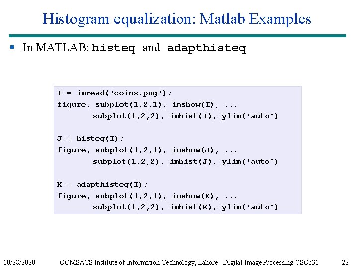
Histogram equalization: Matlab Examples § In MATLAB: histeq and adapthisteq I = imread('coins. png'); figure, subplot(1, 2, 1), imshow(I), . . . subplot(1, 2, 2), imhist(I), ylim('auto') J = histeq(I); figure, subplot(1, 2, 1), imshow(J), . . . subplot(1, 2, 2), imhist(J), ylim('auto') K = adapthisteq(I); figure, subplot(1, 2, 1), imshow(K), . . . subplot(1, 2, 2), imhist(K), ylim('auto') 10/28/2020 COMSATS Institute of Information Technology, Lahore Digital Image Processing CSC 331 22