Chapter 3 Forecasting in POM The Starting Point
- Slides: 52

Chapter 3 Forecasting in POM: The Starting Point for All Planning Slide 0 of 56

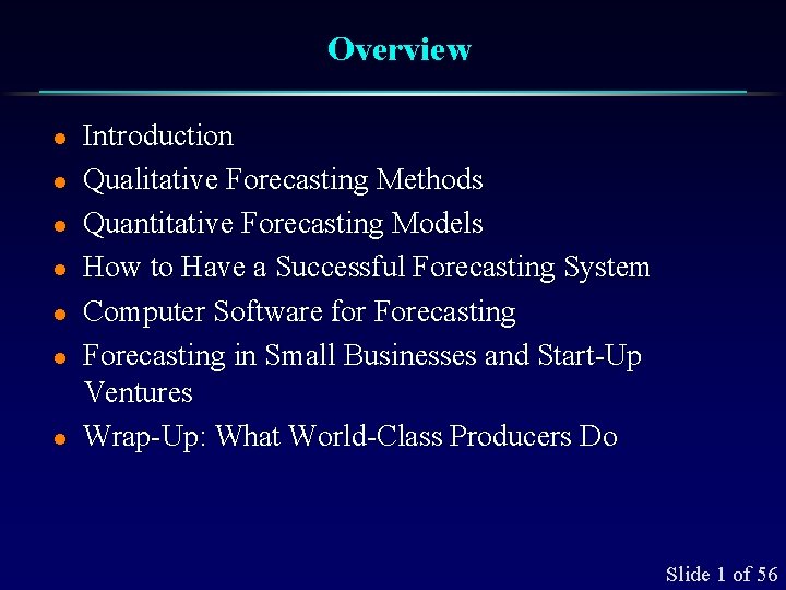
Overview l l l l Introduction Qualitative Forecasting Methods Quantitative Forecasting Models How to Have a Successful Forecasting System Computer Software for Forecasting in Small Businesses and Start-Up Ventures Wrap-Up: What World-Class Producers Do Slide 1 of 56

Demand Management Independent demand items are the only items demand for which needs to be forecast l These items include: l l l Finished goods and Spare parts Slide 2 of 56

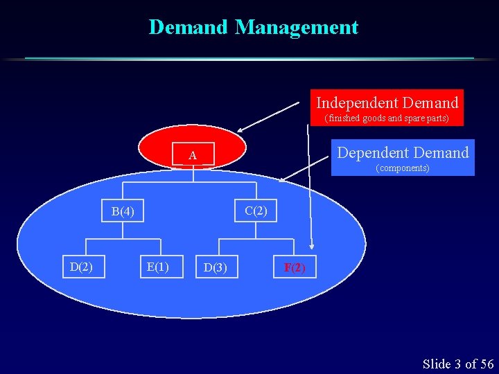
Demand Management Independent Demand (finished goods and spare parts) Dependent Demand A (components) C(2) B(4) D(2) E(1) D(3) F(2) Slide 3 of 56

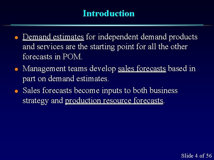
Introduction l l l Demand estimates for independent demand products and services are the starting point for all the other forecasts in POM. Management teams develop sales forecasts based in part on demand estimates. Sales forecasts become inputs to both business strategy and production resource forecasts. Slide 4 of 56

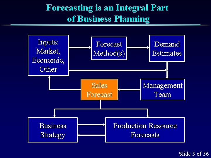
Forecasting is an Integral Part of Business Planning Inputs: Market, Economic, Other Forecast Method(s) Sales Forecast Business Strategy Demand Estimates Management Team Production Resource Forecasts Slide 5 of 56

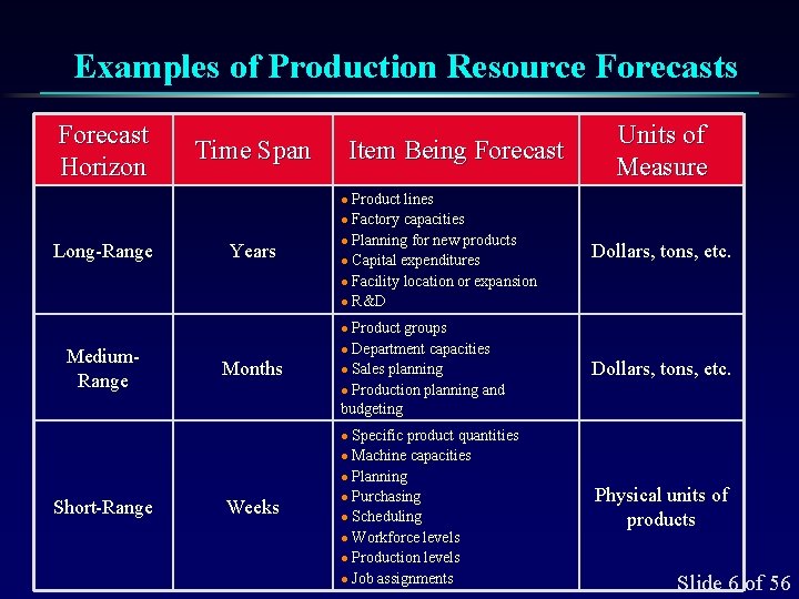
Examples of Production Resource Forecasts Forecast Horizon Time Span Item Being Forecast Units of Measure Product lines l Factory capacities l Planning for new products l Capital expenditures l Facility location or expansion l R&D Dollars, tons, etc. Product groups l Department capacities l Sales planning l Production planning and budgeting Dollars, tons, etc. Specific product quantities l Machine capacities l Planning l Purchasing l Scheduling l Workforce levels l Production levels l Job assignments Physical units of products l Long-Range Years l Medium. Range Months l Short-Range Weeks Slide 6 of 56

Forecasting Methods Qualitative Approaches l Quantitative Approaches l Slide 7 of 56

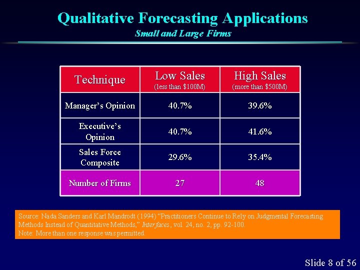
Qualitative Forecasting Applications Small and Large Firms Low Sales High Sales (less than $100 M) (more than $500 M) Manager’s Opinion 40. 7% 39. 6% Executive’s Opinion 40. 7% 41. 6% Sales Force Composite 29. 6% 35. 4% Number of Firms 27 48 Technique Source: Nada Sanders and Karl Mandrodt (1994) “Practitioners Continue to Rely on Judgmental Forecasting Methods Instead of Quantitative Methods, ” Interfaces, vol. 24, no. 2, pp. 92 -100. Note: More than one response was permitted. Slide 8 of 56

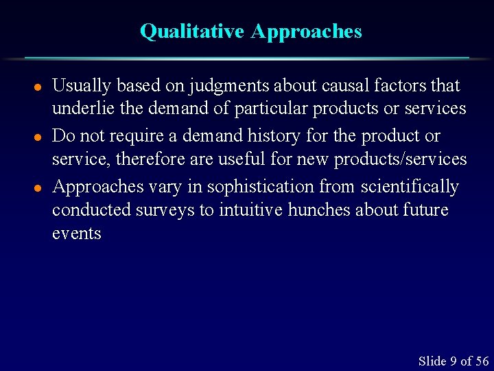
Qualitative Approaches l l l Usually based on judgments about causal factors that underlie the demand of particular products or services Do not require a demand history for the product or service, therefore are useful for new products/services Approaches vary in sophistication from scientifically conducted surveys to intuitive hunches about future events Slide 9 of 56

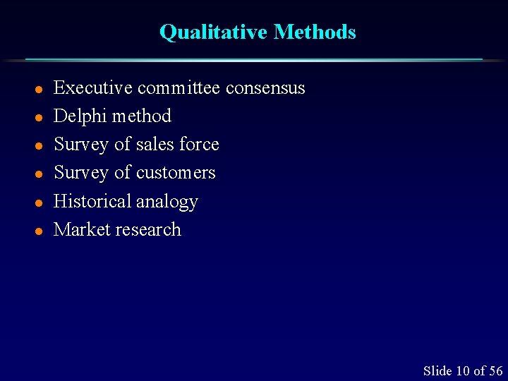
Qualitative Methods l l l Executive committee consensus Delphi method Survey of sales force Survey of customers Historical analogy Market research Slide 10 of 56

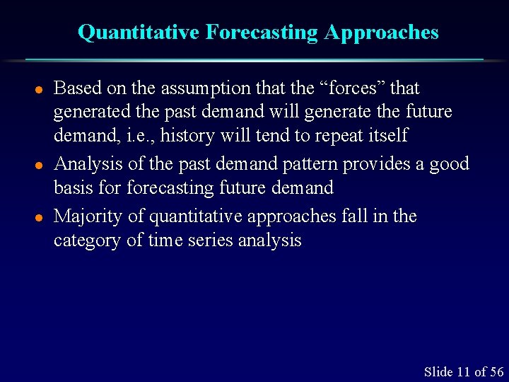
Quantitative Forecasting Approaches l l l Based on the assumption that the “forces” that generated the past demand will generate the future demand, i. e. , history will tend to repeat itself Analysis of the past demand pattern provides a good basis forecasting future demand Majority of quantitative approaches fall in the category of time series analysis Slide 11 of 56

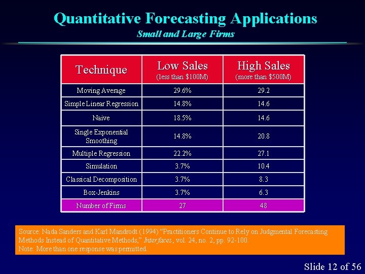
Quantitative Forecasting Applications Small and Large Firms Low Sales High Sales (less than $100 M) (more than $500 M) Moving Average 29. 6% 29. 2 Simple Linear Regression 14. 8% 14. 6 Naive 18. 5% 14. 6 Single Exponential Smoothing 14. 8% 20. 8 Multiple Regression 22. 2% 27. 1 Simulation 3. 7% 10. 4 Classical Decomposition 3. 7% 8. 3 Box-Jenkins 3. 7% 6. 3 Number of Firms 27 48 Technique Source: Nada Sanders and Karl Mandrodt (1994) “Practitioners Continue to Rely on Judgmental Forecasting Methods Instead of Quantitative Methods, ” Interfaces, vol. 24, no. 2, pp. 92 -100. Note: More than one response was permitted. Slide 12 of 56

Time Series Analysis l l l A time series is a set of numbers where the order or sequence of the numbers is important, e. g. , historical demand Analysis of the time series identifies patterns Once the patterns are identified, they can be used to develop a forecast Slide 13 of 56

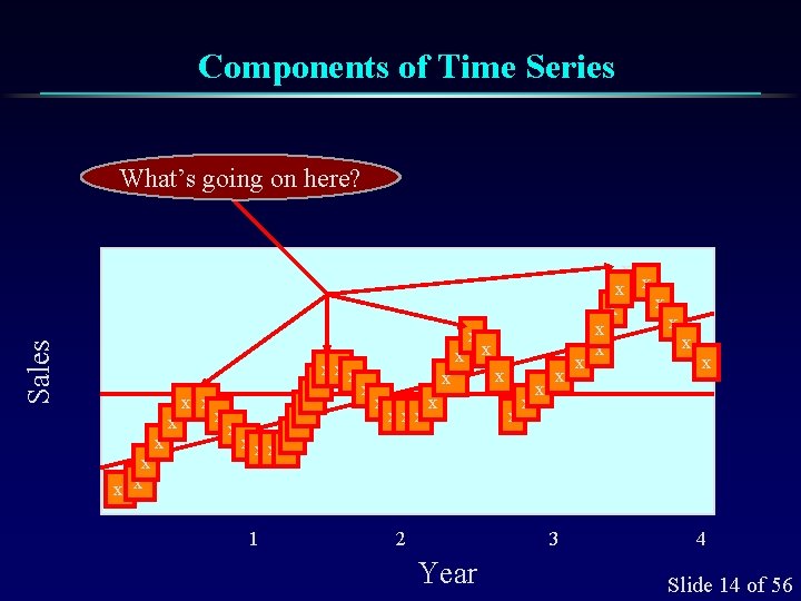
Components of Time Series What’s going on here? Sales x x xx x x x xxxx 1 x x 2 x x x 3 Year x x x 4 Slide 14 of 56

Components of Time Series l l l Trends are noted by an upward or downward sloping line Seasonality is a data pattern that repeats itself over the period of one year or less Cycle is a data pattern that repeats itself. . . may take years Irregular variations are jumps in the level of the series due to extraordinary events Random fluctuation from random variation or unexplained causes Slide 15 of 56

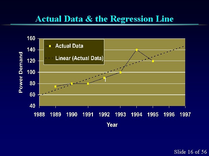
Actual Data & the Regression Line Slide 16 of 56

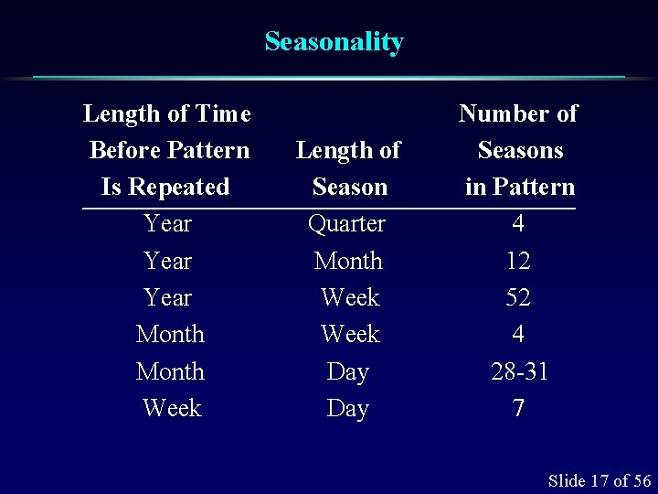
Seasonality Length of Time Before Pattern Is Repeated Year Month Week Length of Season Quarter Month Week Day Number of Seasons in Pattern 4 12 52 4 28 -31 7 Slide 17 of 56

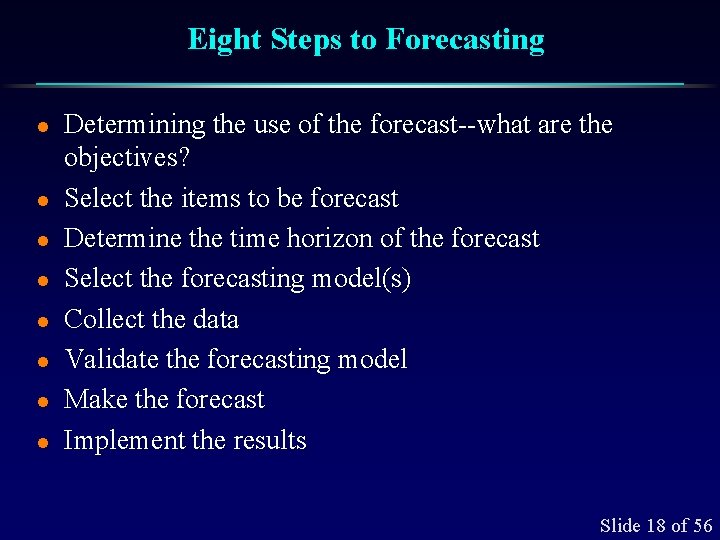
Eight Steps to Forecasting l l l l Determining the use of the forecast--what are the objectives? Select the items to be forecast Determine the time horizon of the forecast Select the forecasting model(s) Collect the data Validate the forecasting model Make the forecast Implement the results Slide 18 of 56

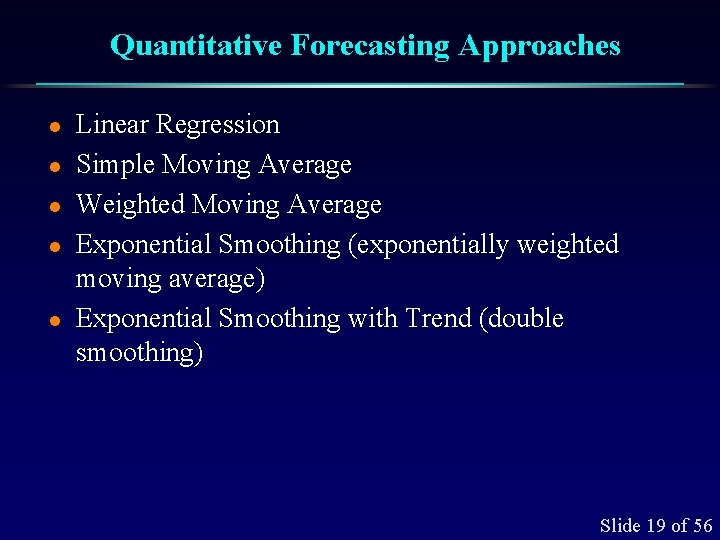
Quantitative Forecasting Approaches l l l Linear Regression Simple Moving Average Weighted Moving Average Exponential Smoothing (exponentially weighted moving average) Exponential Smoothing with Trend (double smoothing) Slide 19 of 56

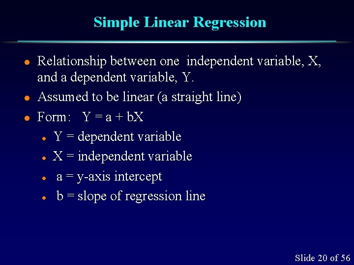
Simple Linear Regression l l l Relationship between one independent variable, X, and a dependent variable, Y. Assumed to be linear (a straight line) Form: Y = a + b. X l Y = dependent variable l X = independent variable l a = y-axis intercept l b = slope of regression line Slide 20 of 56

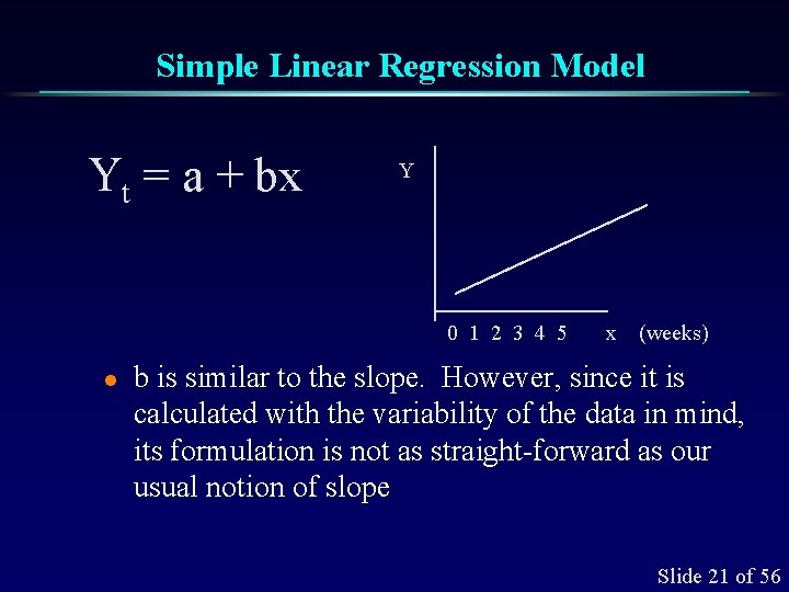
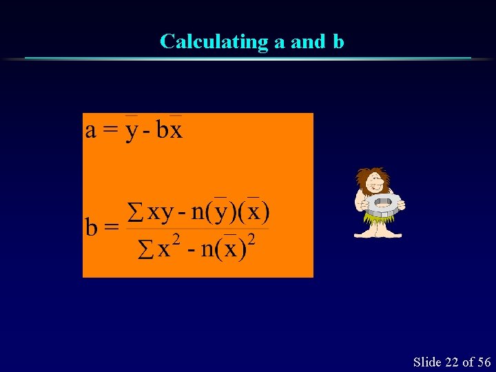
Simple Linear Regression Model Yt = a + bx Y 0 1 2 3 4 5 l x (weeks) b is similar to the slope. However, since it is calculated with the variability of the data in mind, its formulation is not as straight-forward as our usual notion of slope Slide 21 of 56

Calculating a and b Slide 22 of 56

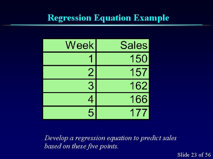
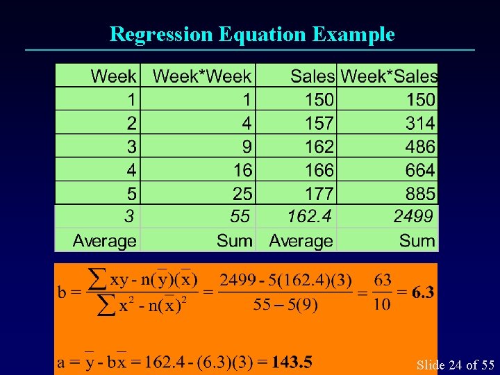
Regression Equation Example Develop a regression equation to predict sales based on these five points. Slide 23 of 56

Regression Equation Example Slide 24 of 55

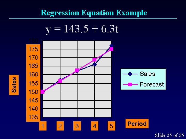
Regression Equation Example Sales y = 143. 5 + 6. 3 t 180 175 170 165 160 155 150 145 140 135 Sales Forecast 1 2 3 4 5 Period Slide 25 of 55

Forecast Accuracy l l Accuracy is the typical criterion for judging the performance of a forecasting approach Accuracy is how well the forecasted values match the actual values Slide 26 of 56

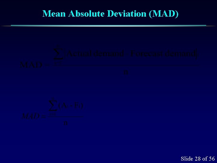
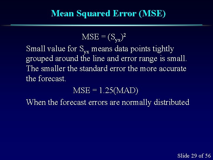
Monitoring Accuracy l l Accuracy of a forecasting approach needs to be monitored to assess the confidence you can have in its forecasts and changes in the market may require reevaluation of the approach Accuracy can be measured in several ways l Mean absolute deviation (MAD) l Mean squared error (MSE) Slide 27 of 56

Mean Absolute Deviation (MAD) Slide 28 of 56

Mean Squared Error (MSE) MSE = (Syx)2 Small value for Syx means data points tightly grouped around the line and error range is small. The smaller the standard error the more accurate the forecast. MSE = 1. 25(MAD) When the forecast errors are normally distributed Slide 29 of 56

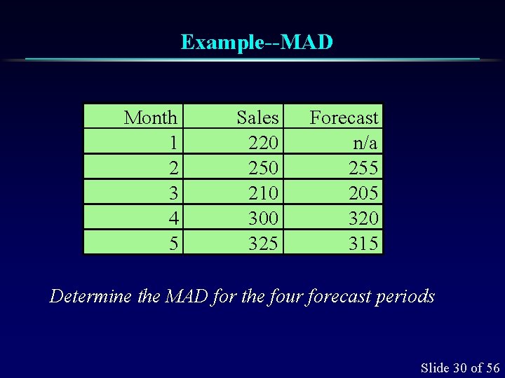
Example--MAD Month 1 2 3 4 5 Sales 220 250 210 300 325 Forecast n/a 255 205 320 315 Determine the MAD for the four forecast periods Slide 30 of 56

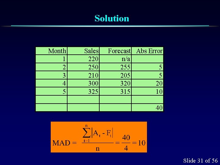
Solution Month 1 2 3 4 5 Sales 220 250 210 300 325 Forecast Abs Error n/a 255 5 205 5 320 20 315 10 40 Slide 31 of 56

Simple Moving Average l l An averaging period (AP) is given or selected The forecast for the next period is the arithmetic average of the AP most recent actual demands It is called a “simple” average because each period used to compute the average is equally weighted. . . more Slide 32 of 56

Simple Moving Average l l l It is called “moving” because as new demand data becomes available, the oldest data is not used By increasing the AP, the forecast is less responsive to fluctuations in demand (low impulse response) By decreasing the AP, the forecast is more responsive to fluctuations in demand (high impulse response) Slide 33 of 56

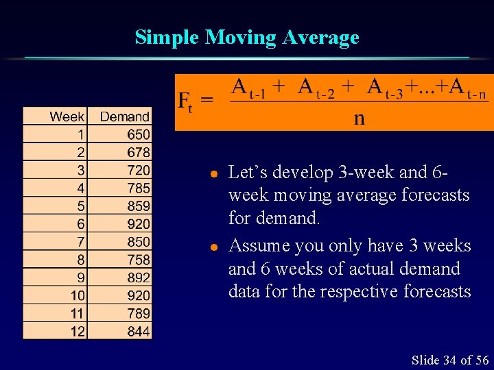
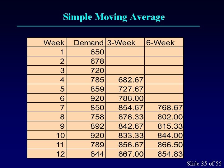
Simple Moving Average l l Let’s develop 3 -week and 6 week moving average forecasts for demand. Assume you only have 3 weeks and 6 weeks of actual demand data for the respective forecasts Slide 34 of 56

Simple Moving Average Slide 35 of 55

Simple Moving Average Slide 36 of 55

Weighted Moving Average l l l This is a variation on the simple moving average where instead of the weights used to compute the average being equal, they are not equal This allows more recent demand data to have a greater effect on the moving average, therefore the forecast. . . more Slide 37 of 56

Weighted Moving Average l l The weights must add to 1. 0 and generally decrease in value with the age of the data The distribution of the weights determine impulse response of the forecast Slide 38 of 56

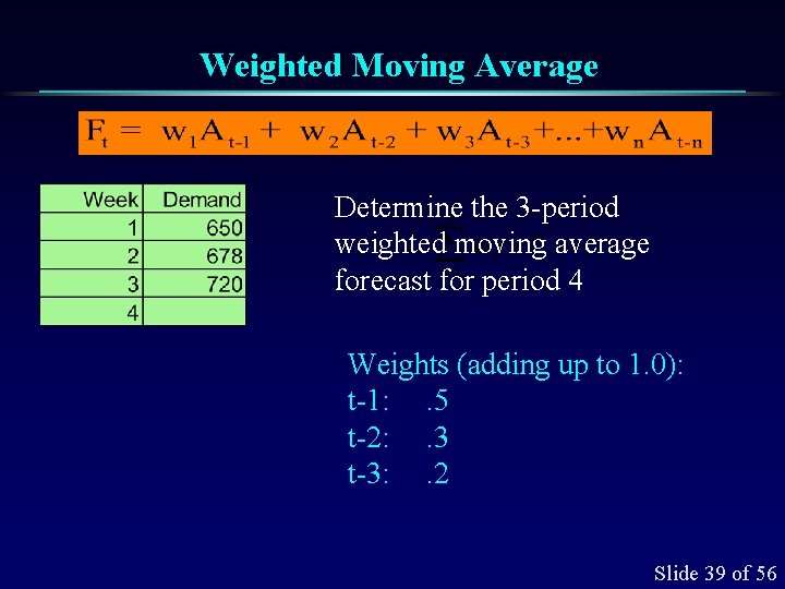
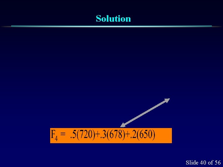
Weighted Moving Average Determine the 3 -period weighted moving average forecast for period 4 Weights (adding up to 1. 0): t-1: . 5 t-2: . 3 t-3: . 2 Slide 39 of 56

Solution Slide 40 of 56

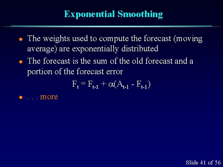
Exponential Smoothing l l l The weights used to compute the forecast (moving average) are exponentially distributed The forecast is the sum of the old forecast and a portion of the forecast error Ft = Ft-1 + (At-1 - Ft-1). . . more Slide 41 of 56

Exponential Smoothing l l l The smoothing constant, , must be between 0. 0 and 1. 0 (excluding 0. 0 and 1. 0) A large provides a high impulse response forecast A small provides a low impulse response forecast Slide 42 of 56

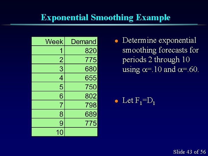
Exponential Smoothing Example l l Determine exponential smoothing forecasts for periods 2 through 10 using =. 10 and =. 60. Let F 1=D 1 Slide 43 of 56

Exponential Smoothing Example Slide 44 of 55

Effect of on Forecast Slide 45 of 56

Criteria for Selecting a Forecasting Method l l l Cost Accuracy Data available Time span Nature of products and services Impulse response and noise dampening Slide 46 of 56

Reasons for Ineffective Forecasting l l l Not involving a broad cross section of people Not recognizing that forecasting is integral to business planning Not recognizing that forecasts will always be wrong (think in terms of interval rather than point forecasts) Not forecasting the right things (forecast independent demand only) Not selecting an appropriate forecasting method (use MAD to evaluate goodness of fit) Not tracking the accuracy of the forecasting models Slide 47 of 56

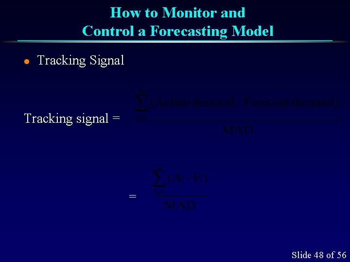
How to Monitor and Control a Forecasting Model l Tracking Signal Tracking signal = = Slide 48 of 56

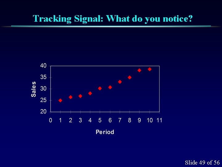
Tracking Signal: What do you notice? Slide 49 of 56

Sources of Forecasting Data l l l l Consumer Confidence Index Consumer Price Index Housing Starts Index of Leading Economic Indicators Personal Income and Consumption Producer Price Index Purchasing Manager’s Index Retail Sales Slide 50 of 56

Wrap-Up: World-Class Practice l l l Predisposed to have effective methods of forecasting because they have exceptional long-range business planning Formal forecasting effort Develop methods to monitor the performance of their forecasting models Use forecasting software with automated model fitting features, which is readily available today Do not overlook the short run. . excellent short range forecasts as well Slide 51 of 56