CHAPTER 13 FORECASTING Outline Forecasting and Choice of

CHAPTER 13 FORECASTING Outline • Forecasting and Choice of a Forecasting Methods • Methods for Stationary Series: – Simple and Weighted Moving Average – Exponential smoothing • Trend-Based Methods – Regression – Double Exponential Smoothing: Holt’s Method • A Method for Seasonality and Trend

Forecasting

Decisions Based on Forecasts • Production – Aggregate planning, inventory control, scheduling • Marketing – New product introduction, salesforce allocation, promotions • Finance – Plant/equipment investment, budgetary planning • Personnel – Workforce planning, hiring, layoff

Characteristics of Forecasts • Forecasts are always wrong; so consider both expected value and a measure of forecast error • Long-term forecasts are less accurate than short-term forecasts • Aggregate forecasts are more accurate than disaggregate forecasts

Forecasting • • Components of demand Evaluation of forecasts Time series: stationary series Time series: trend – Linear regression – Double exponential smoothing • Time series: seasonality

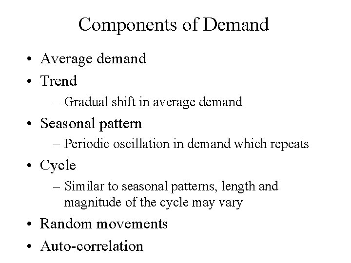
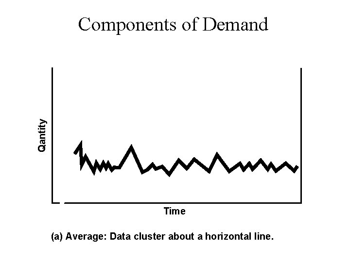
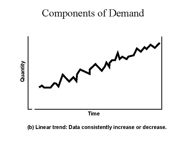
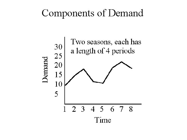
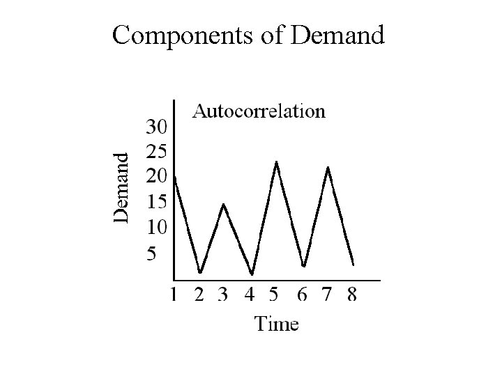
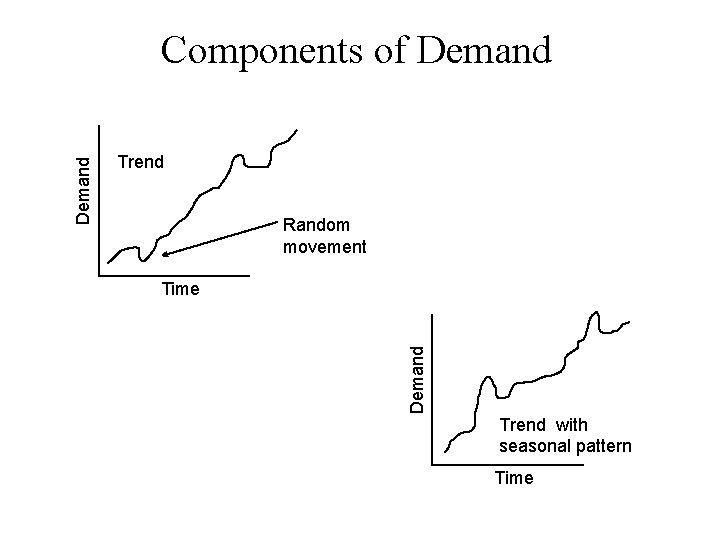
Components of Demand • Average demand • Trend – Gradual shift in average demand • Seasonal pattern – Periodic oscillation in demand which repeats • Cycle – Similar to seasonal patterns, length and magnitude of the cycle may vary • Random movements • Auto-correlation

Qantity Components of Demand Time (a) Average: Data cluster about a horizontal line.

Quantity Components of Demand Time (b) Linear trend: Data consistently increase or decrease.

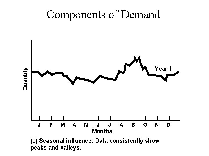
Components of Demand Quantity Year 1 | | | J F M A M J J A S O N D Months (c) Seasonal influence: Data consistently show peaks and valleys.

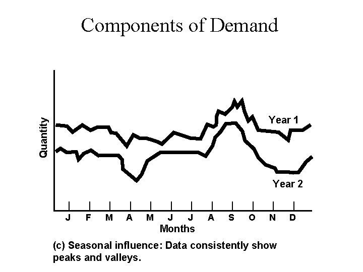
Components of Demand Quantity Year 1 Year 2 | | | J F M A M J J A S O N D Months (c) Seasonal influence: Data consistently show peaks and valleys.

Components of Demand

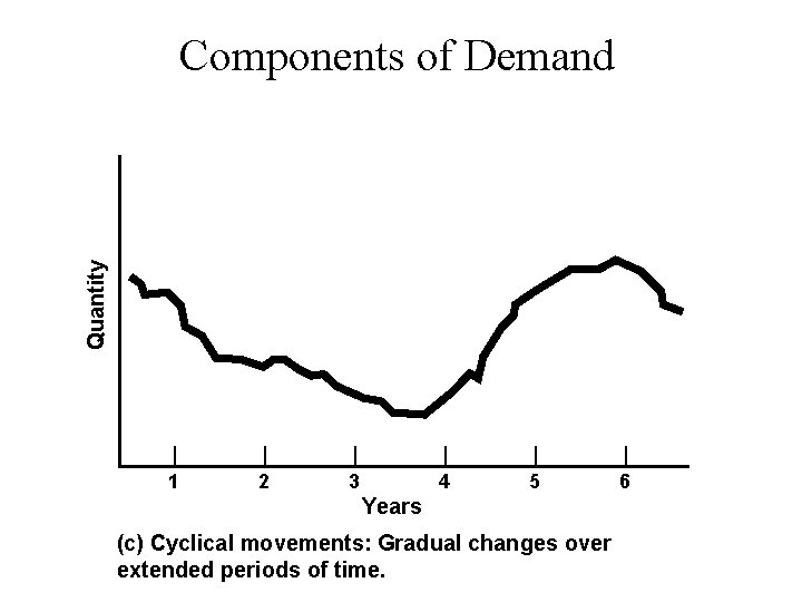
Quantity Components of Demand | | | 1 2 3 4 5 6 Years (c) Cyclical movements: Gradual changes over extended periods of time.

Components of Demand

Trend Random movement Time Demand Components of Demand Trend with seasonal pattern Time

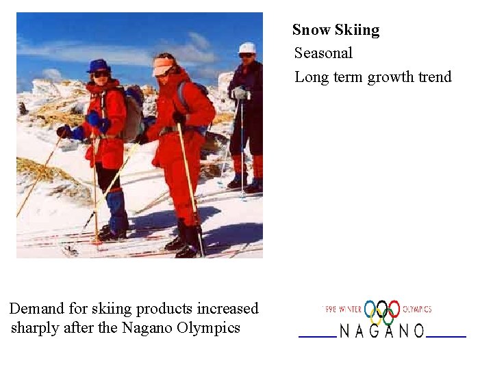
Snow Skiing Seasonal Long term growth trend Demand for skiing products increased sharply after the Nagano Olympics

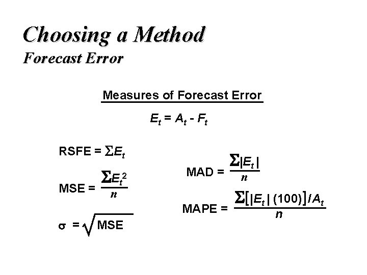
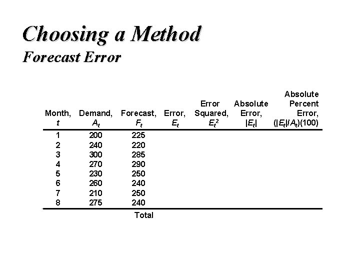
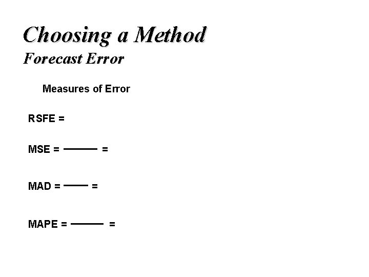
Choosing a Method Forecast Error Measures of Forecast Error E t = At - F t RSFE = Et MSE = E t 2 MAD = n MAPE = = MSE |Et | n [ |Et | (100) ] / At n

Choosing a Method Forecast Error Month, Demand, t At 1 2 3 4 5 6 7 8 200 240 300 270 230 260 210 275 Forecast, Error, Ft Et 225 220 285 290 250 240 - Total Absolute Error Absolute Percent Squared, Error, 2 Et |Et| (|Et|/At)(100)

Choosing a Method Forecast Error Measures of Error RSFE = MSE = MAD = MAPE = =

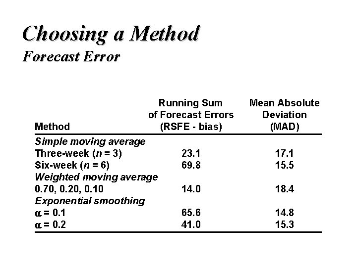
Choosing a Method Forecast Error Running Sum of Forecast Errors (RSFE - bias) Mean Absolute Deviation (MAD) 23. 1 69. 8 17. 1 15. 5 14. 0 18. 4 65. 6 41. 0 14. 8 15. 3 Method Simple moving average Three-week (n = 3) Six-week (n = 6) Weighted moving average 0. 70, 0. 20, 0. 10 Exponential smoothing = 0. 1 = 0. 2

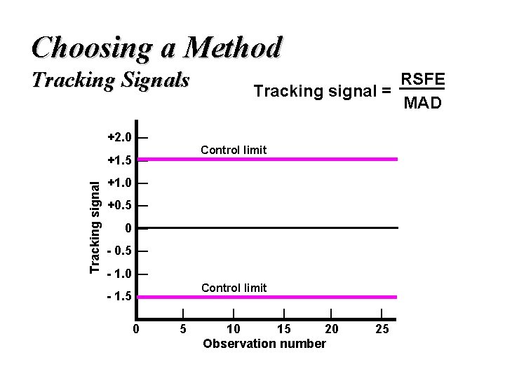
Choosing a Method Tracking Signals +2. 0 — Control limit +1. 5 — Tracking signal RSFE Tracking signal = MAD +1. 0 — +0. 5 — 0— - 0. 5 — - 1. 0 — Control limit - 1. 5 — 0 | 5 | | | 10 15 20 Observation number | 25

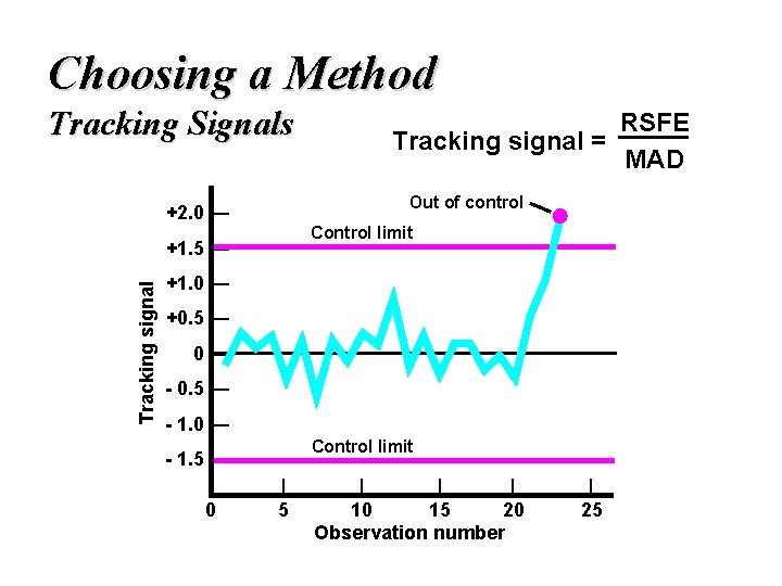
Choosing a Method Tracking Signals Out of control +2. 0 — Control limit +1. 5 — Tracking signal RSFE Tracking signal = MAD +1. 0 — +0. 5 — 0— - 0. 5 — - 1. 0 — Control limit - 1. 5 — 0 | 5 | | | 10 15 20 Observation number | 25

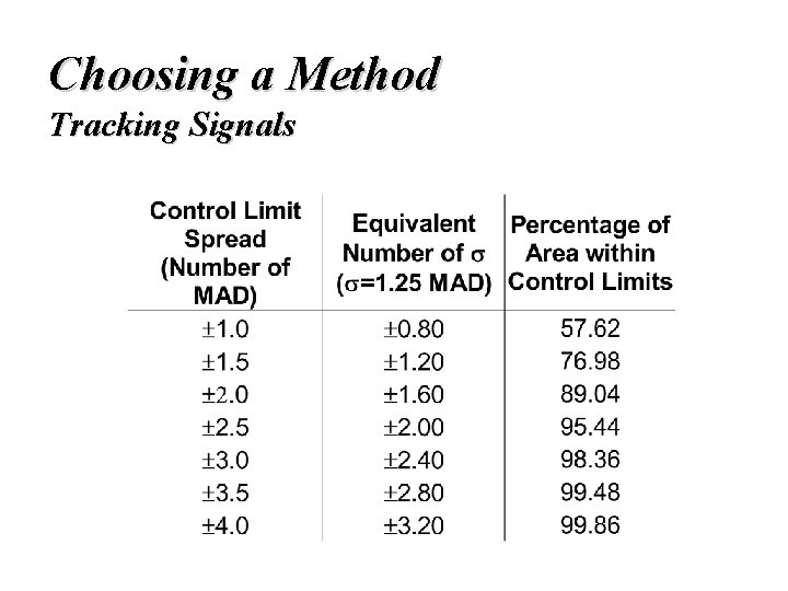
Choosing a Method Tracking Signals

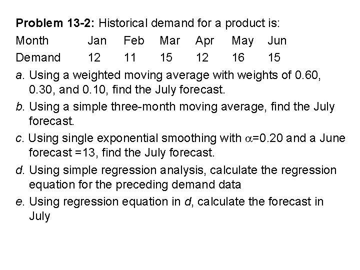
Problem 13 -2: Historical demand for a product is: Month Jan Feb Mar Apr May Jun Demand 12 11 15 12 16 15 a. Using a weighted moving average with weights of 0. 60, 0. 30, and 0. 10, find the July forecast. b. Using a simple three-month moving average, find the July forecast. c. Usingle exponential smoothing with =0. 20 and a June forecast =13, find the July forecast. d. Using simple regression analysis, calculate the regression equation for the preceding demand data e. Using regression equation in d, calculate the forecast in July

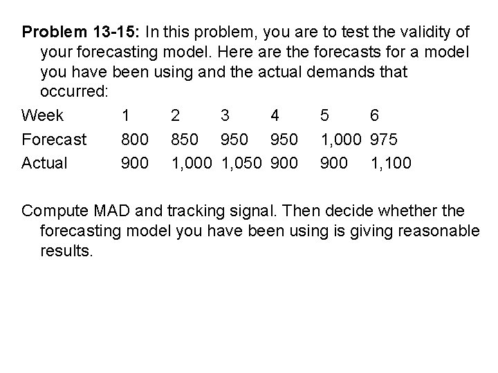
Problem 13 -15: In this problem, you are to test the validity of your forecasting model. Here are the forecasts for a model you have been using and the actual demands that occurred: Week 1 2 3 4 5 6 Forecast 800 850 950 1, 000 975 Actual 900 1, 050 900 1, 100 Compute MAD and tracking signal. Then decide whether the forecasting model you have been using is giving reasonable results.

Methods for Stationary Series

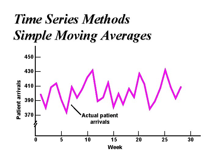
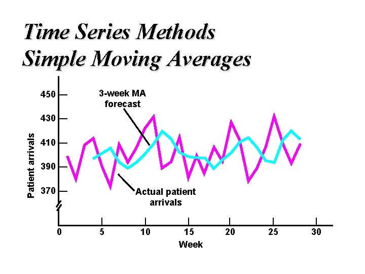
Time Series Methods Simple Moving Averages 450 — Patient arrivals 430 — 410 — 390 — 370 — 0 Actual patient arrivals | 5 | 10 | 15 Week | 20 | 25 | 30

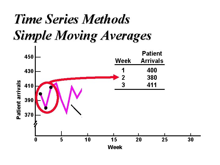
Time Series Methods Simple Moving Averages 450 — Week Patient Arrivals 1 2 3 400 380 411 Patient arrivals 430 — 410 — 390 — 370 — 0 Actual patient arrivals | 5 | 10 | 15 Week | 20 | 25 | 30

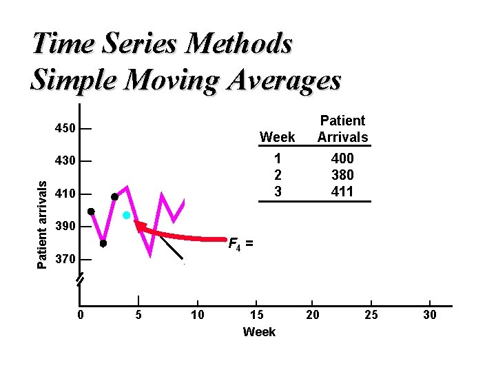
Time Series Methods Simple Moving Averages 450 — Week Patient Arrivals 1 2 3 400 380 411 Patient arrivals 430 — 410 — 390 — F 4 = 370 — 0 Actual patient arrivals | 5 | 10 | 15 Week | 20 | 25 | 30

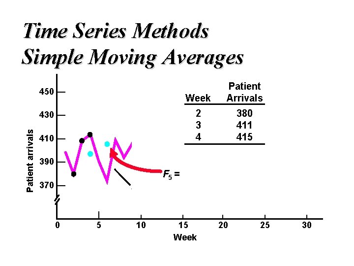
Time Series Methods Simple Moving Averages 450 — Week Patient Arrivals 2 3 4 380 411 415 Patient arrivals 430 — 410 — 390 — F 5 = 370 — 0 Actual patient arrivals | 5 | 10 | 15 Week | 20 | 25 | 30

Time Series Methods Simple Moving Averages 450 — 3 -week MA forecast Patient arrivals 430 — 410 — 390 — 370 — 0 Actual patient arrivals | 5 | 10 | 15 Week | 20 | 25 | 30

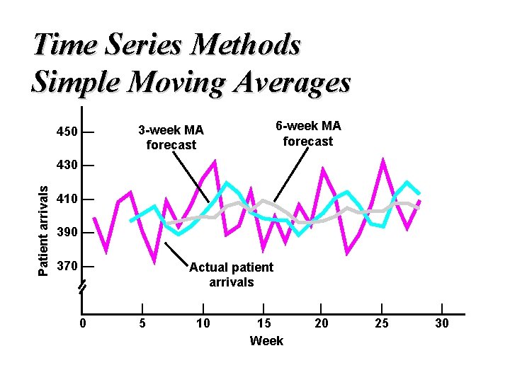
Time Series Methods Simple Moving Averages 450 — 6 -week MA forecast 3 -week MA forecast Patient arrivals 430 — 410 — 390 — 370 — 0 Actual patient arrivals | 5 | 10 | 15 Week | 20 | 25 | 30

Taco Bell determined that the demand for each 15 minute interval can be estimated from a 6 week simple moving average of sales. The forecast was used to determine the number of employees needed.

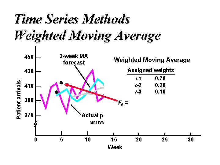
Time Series Methods Weighted Moving Average 450 — 3 -week MA forecast Weighted Moving Average Assigned weights Patient arrivals 430 — t-1 t-2 t-3 410 — 390 — F 4 = 370 — 0 0. 70 0. 20 0. 10 Actual patient arrivals | 5 | 10 | 15 Week | 20 | 25 | 30

Time Series Methods Weighted Moving Average 450 — 3 -week MA forecast Weighted Moving Average Assigned weights Patient arrivals 430 — t-1 t-2 t-3 410 — 390 — F 5 = 370 — 0 0. 70 0. 20 0. 10 Actual patient arrivals | 5 | 10 | 15 Week | 20 | 25 | 30

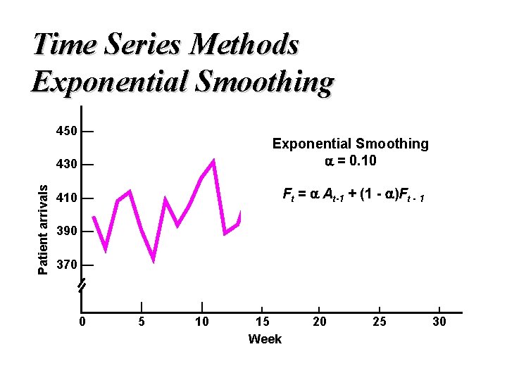
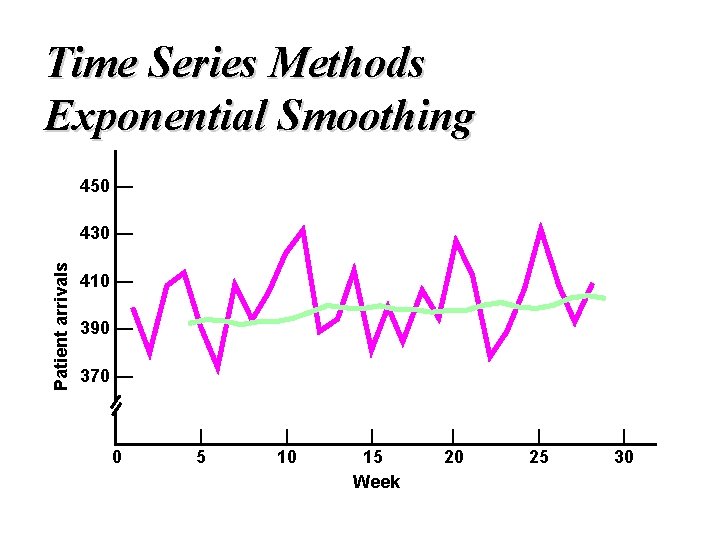
Time Series Methods Exponential Smoothing Patient arrivals 450 — 430 — Exponential Smoothing = 0. 10 410 — Ft = At-1 + (1 - )Ft - 1 390 — 370 — 0 | 5 | 10 | 15 Week | 20 | 25 | 30

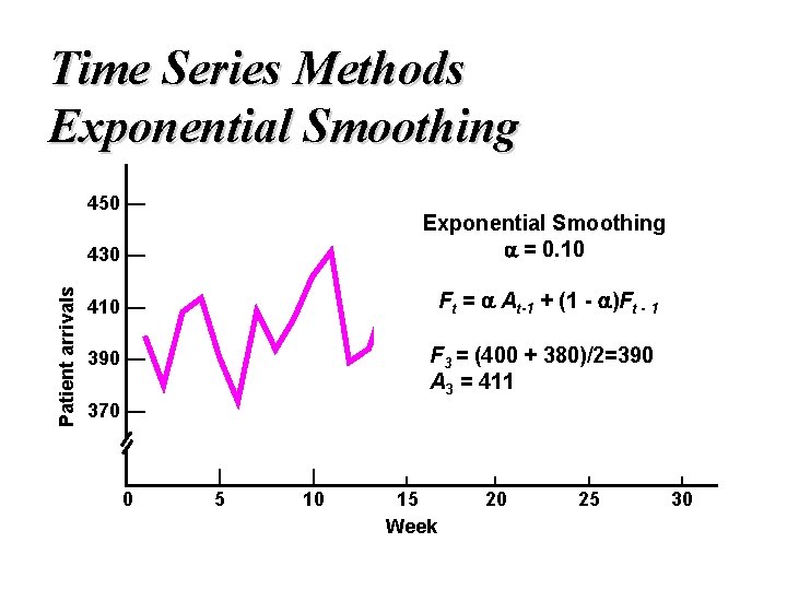
Time Series Methods Exponential Smoothing Patient arrivals 450 — 430 — Exponential Smoothing = 0. 10 410 — Ft = At-1 + (1 - )Ft - 1 F 3 = (400 + 380)/2=390 A 3 = 411 390 — 370 — 0 | 5 | 10 | 15 Week | 20 | 25 | 30

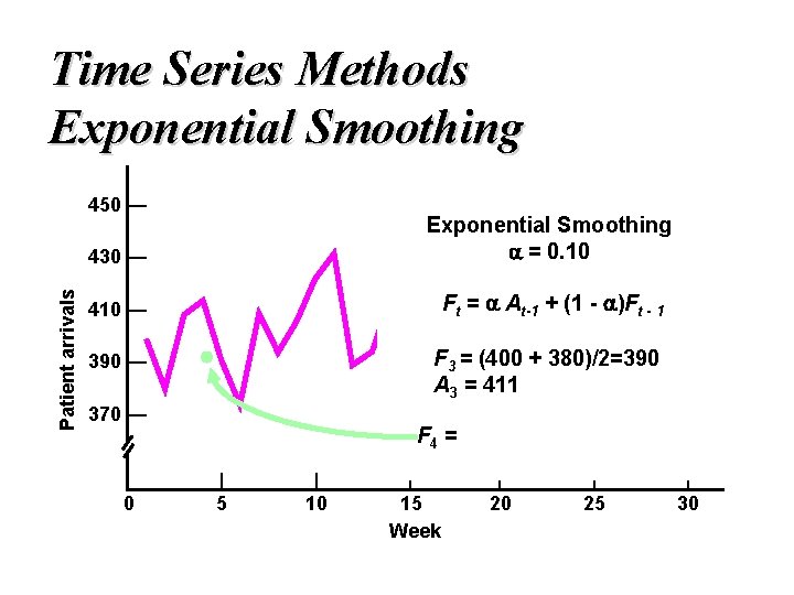
Time Series Methods Exponential Smoothing Patient arrivals 450 — 430 — Exponential Smoothing = 0. 10 410 — Ft = At-1 + (1 - )Ft - 1 F 3 = (400 + 380)/2=390 A 3 = 411 390 — 370 — 0 F 4 = | 5 | 10 | 15 Week | 20 | 25 | 30

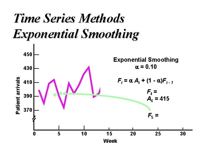
Time Series Methods Exponential Smoothing Patient arrivals 450 — 430 — Exponential Smoothing = 0. 10 410 — Ft = At + (1 - )Ft - 1 F 4 = A 4 = 415 390 — 370 — 0 F 5 = | 5 | 10 | 15 Week | 20 | 25 | 30

Time Series Methods Exponential Smoothing 450 — Patient arrivals 430 — 410 — 390 — 370 — 0 | 5 | 10 | 15 Week | 20 | 25 | 30

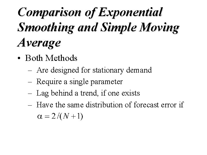
Comparison of Exponential Smoothing and Simple Moving Average • Both Methods – – Are designed for stationary demand Require a single parameter Lag behind a trend, if one exists Have the same distribution of forecast error if

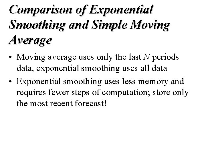
Comparison of Exponential Smoothing and Simple Moving Average • Moving average uses only the last N periods data, exponential smoothing uses all data • Exponential smoothing uses less memory and requires fewer steps of computation; store only the most recent forecast!

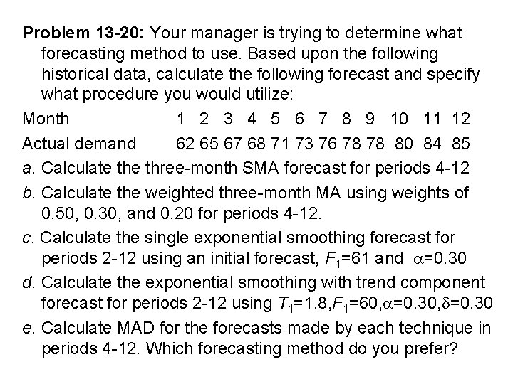
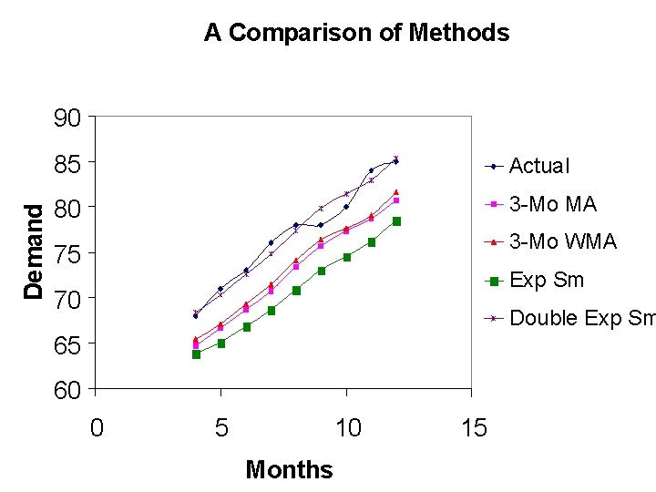
Problem 13 -20: Your manager is trying to determine what forecasting method to use. Based upon the following historical data, calculate the following forecast and specify what procedure you would utilize: Month 1 2 3 4 5 6 7 8 9 10 11 12 Actual demand 62 65 67 68 71 73 76 78 78 80 84 85 a. Calculate three-month SMA forecast for periods 4 -12 b. Calculate the weighted three-month MA using weights of 0. 50, 0. 30, and 0. 20 for periods 4 -12. c. Calculate the single exponential smoothing forecast for periods 2 -12 using an initial forecast, F 1=61 and =0. 30 d. Calculate the exponential smoothing with trend component forecast for periods 2 -12 using T 1=1. 8, F 1=60, =0. 30 e. Calculate MAD for the forecasts made by each technique in periods 4 -12. Which forecasting method do you prefer?

Trend-Based Methods

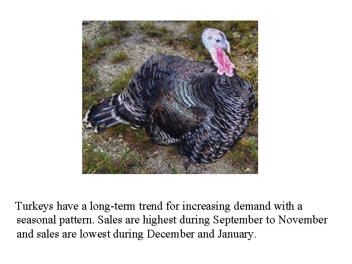
Turkeys have a long-term trend for increasing demand with a seasonal pattern. Sales are highest during September to November and sales are lowest during December and January.

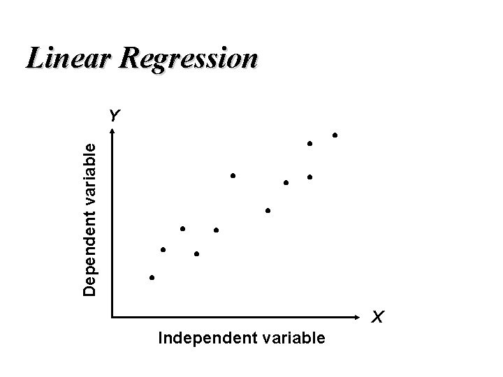
Linear Regression Dependent variable Y X Independent variable

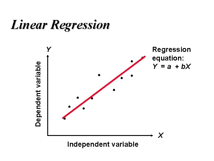
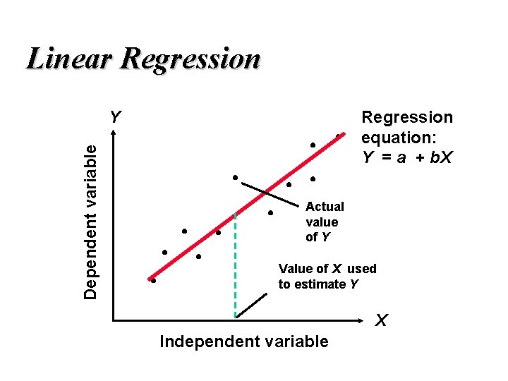
Linear Regression equation: Y = a + b. X Dependent variable Y X Independent variable

Linear Regression equation: Y = a + b. X Dependent variable Y Actual value of Y Value of X used to estimate Y X Independent variable

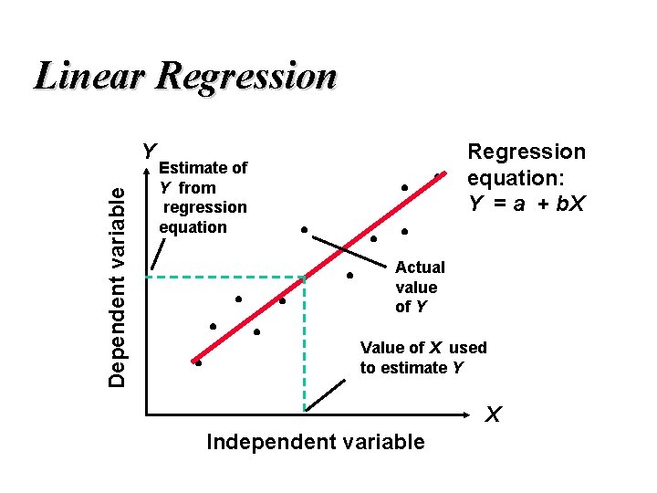
Linear Regression Dependent variable Y Regression equation: Y = a + b. X Estimate of Y from regression equation Actual value of Y Value of X used to estimate Y X Independent variable

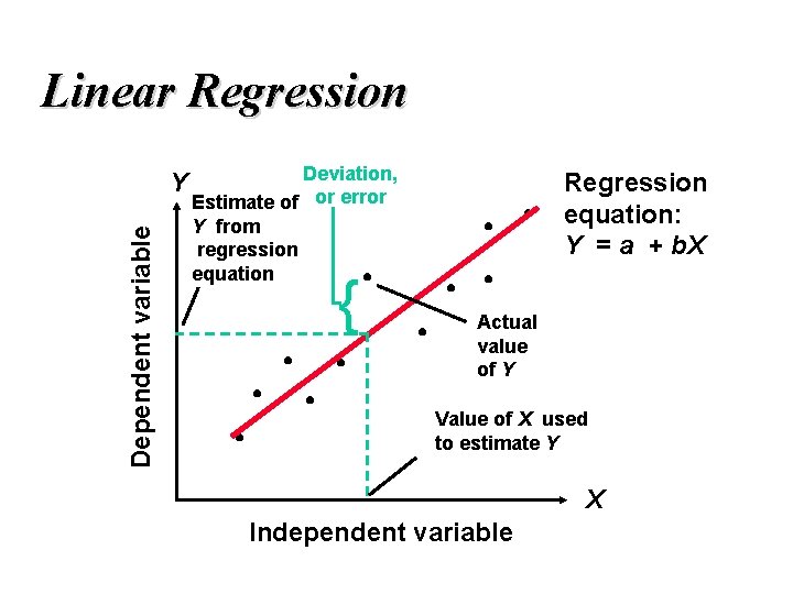
Linear Regression Dependent variable Y Deviation, Estimate of or error Y from regression equation { Regression equation: Y = a + b. X Actual value of Y Value of X used to estimate Y X Independent variable

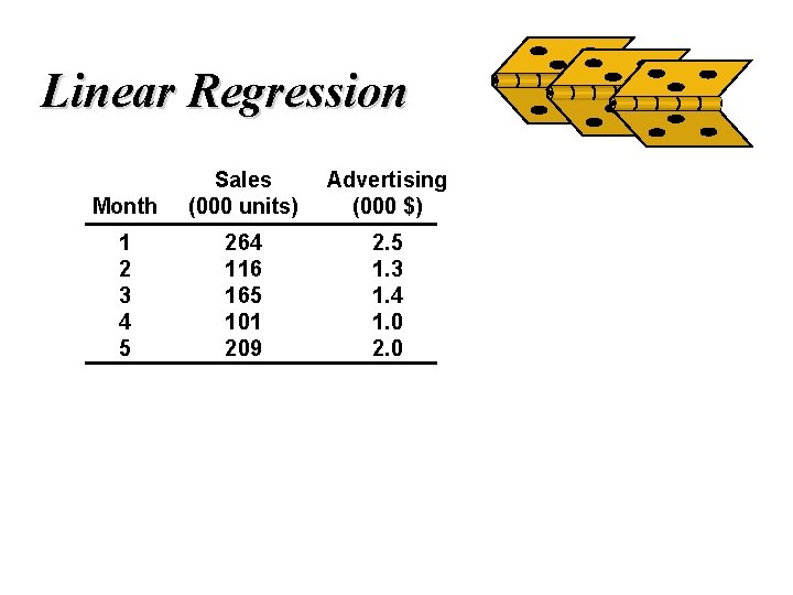
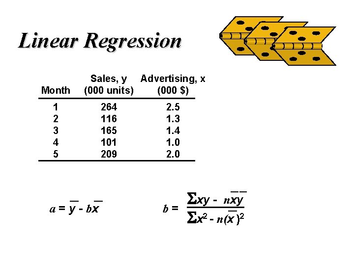
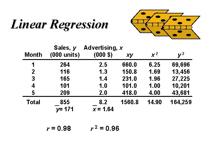
Linear Regression Month Sales (000 units) Advertising (000 $) 1 2 3 4 5 264 116 165 101 209 2. 5 1. 3 1. 4 1. 0 2. 0

Linear Regression Month Sales, y Advertising, x (000 units) (000 $) 1 2 3 4 5 a = y - bx 264 116 165 101 209 2. 5 1. 3 1. 4 1. 0 2. 0 b= xy - nxy x 2 - n(x )2

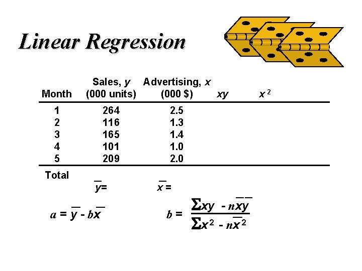
Linear Regression Month Sales, y Advertising, x (000 units) (000 $) xy 1 2 3 4 5 264 116 165 101 209 2. 5 1. 3 1. 4 1. 0 2. 0 Total y= a = y - bx x= b= xy - nxy x 2 - nx 2

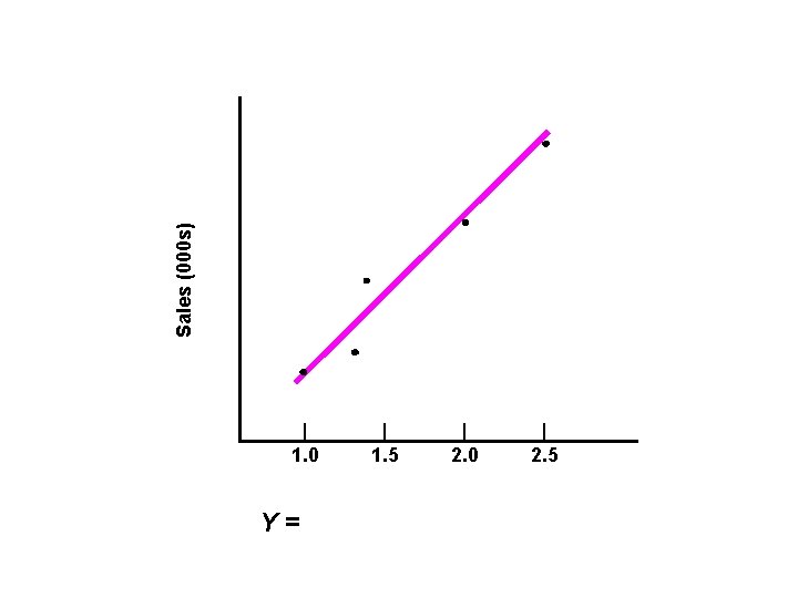
300 — Sales (000 s) 250 — 200 — 150 — 100 — 50 | 1. 0 Y= | 1. 5 | 2. 0 b = 109. 229 | 2. 5

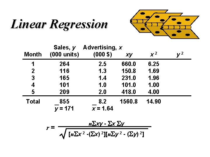
Linear Regression Month Sales, y Advertising, x (000 units) (000 $) xy x 2 1 2 3 4 5 264 116 165 101 209 2. 5 1. 3 1. 4 1. 0 2. 0 660. 0 150. 8 231. 0 101. 0 418. 0 6. 25 1. 69 1. 96 1. 00 4. 00 Total 855 y = 171 8. 2 x = 1. 64 1560. 8 14. 90 r= n xy - x y [n x 2 -( x) 2][n y 2 - ( y) 2] y 2

Linear Regression Month Sales, y Advertising, x (000 units) (000 $) xy x 2 y 2 1 2 3 4 5 264 116 165 101 209 2. 5 1. 3 1. 4 1. 0 2. 0 660. 0 150. 8 231. 0 101. 0 418. 0 6. 25 1. 69 1. 96 1. 00 4. 00 69, 696 13, 456 27, 225 10, 201 43, 681 Total 855 y= 171 8. 2 x = 1. 64 1560. 8 14. 90 164, 259 r = 0. 98 r 2 = 0. 96

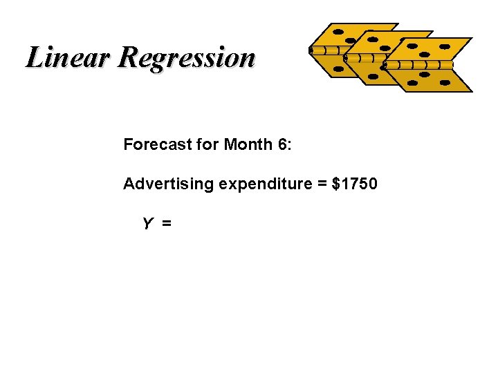
Linear Regression Forecast for Month 6: Advertising expenditure = $1750 Y =

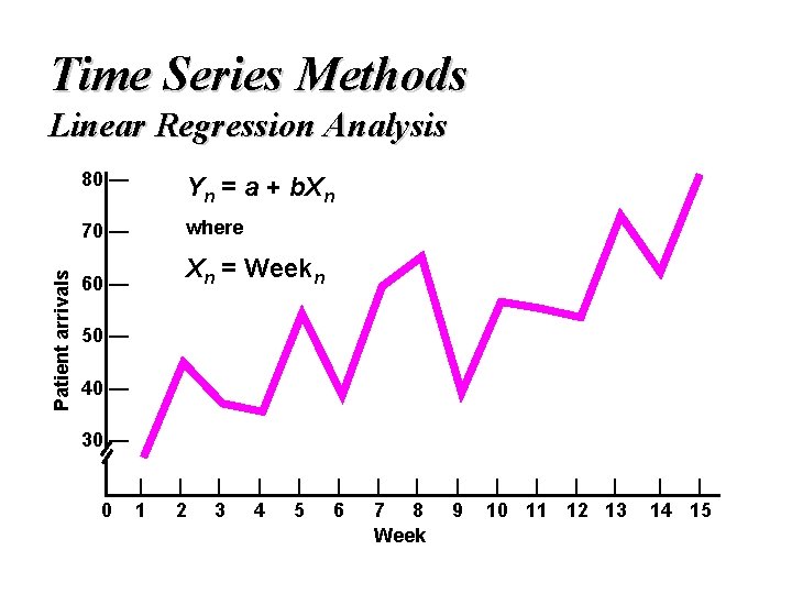
Time Series Methods Patient arrivals Linear Regression Analysis 80 — Yn = a + b. Xn 70 — where 60 — Xn = Weekn 50 — 40 — 30 — 0 | 1 | 2 | 3 | 4 | 5 | 6 | | 7 8 Week | 9 | | 10 11 12 13 | | 14 15

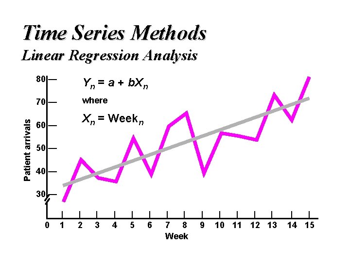
Time Series Methods Patient arrivals Linear Regression Analysis 80 — Yn = a + b. Xn 70 — where 60 — Xn = Weekn 50 — 40 — 30 — 0 | 1 | 2 | 3 | 4 | 5 | 6 | | 7 8 Week | 9 | | 10 11 12 13 | | 14 15

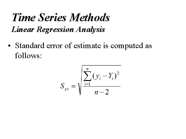
Time Series Methods Linear Regression Analysis • Standard error of estimate is computed as follows:

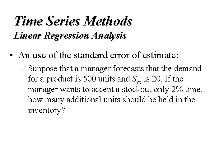
Time Series Methods Linear Regression Analysis • An use of the standard error of estimate: – Suppose that a manager forecasts that the demand for a product is 500 units and Syx is 20. If the manager wants to accept a stockout only 2% time, how many additional units should be held in the inventory?

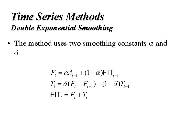
Time Series Methods Double Exponential Smoothing • The method uses two smoothing constants and

A Comparison of Methods Demand 90 85 Actual 80 3 -Mo MA 3 -Mo WMA 75 Exp Sm 70 Double Exp Sm 65 60 0 5 10 Months 15

Methods for Seasonal Series

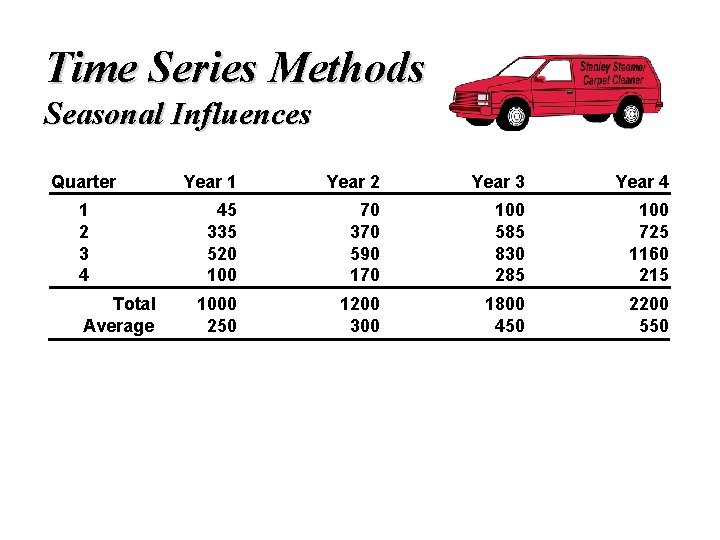
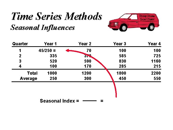
Time Series Methods Seasonal Influences Quarter 1 2 3 4 Total Average Year 1 Year 2 Year 3 Year 4 45 335 520 100 70 370 590 170 100 585 830 285 100 725 1160 215 1000 250 1200 300 1800 450 2200 550

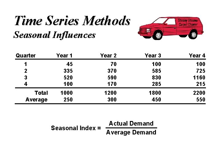
Time Series Methods Seasonal Influences Quarter 1 2 3 4 Total Average Year 1 Year 2 Year 3 Year 4 45 335 520 100 70 370 590 170 100 585 830 285 100 725 1160 215 1000 250 1200 300 1800 450 2200 550 Actual Demand Seasonal Index = Average Demand

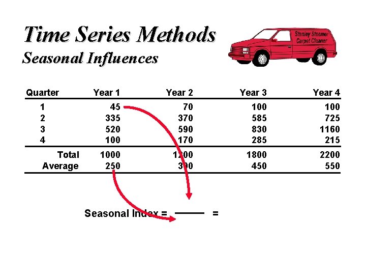
Time Series Methods Seasonal Influences Quarter 1 2 3 4 Total Average Year 1 Year 2 Year 3 Year 4 45 335 520 100 70 370 590 170 100 585 830 285 100 725 1160 215 1000 250 1200 300 1800 450 2200 550 Seasonal Index = =

Time Series Methods Seasonal Influences Quarter 1 2 3 4 Total Average Year 1 Year 2 Year 3 Year 4 45/250 = 335 520 100 70 370 590 170 100 585 830 285 100 725 1160 215 1000 250 1200 300 1800 450 2200 550 Seasonal Index = =

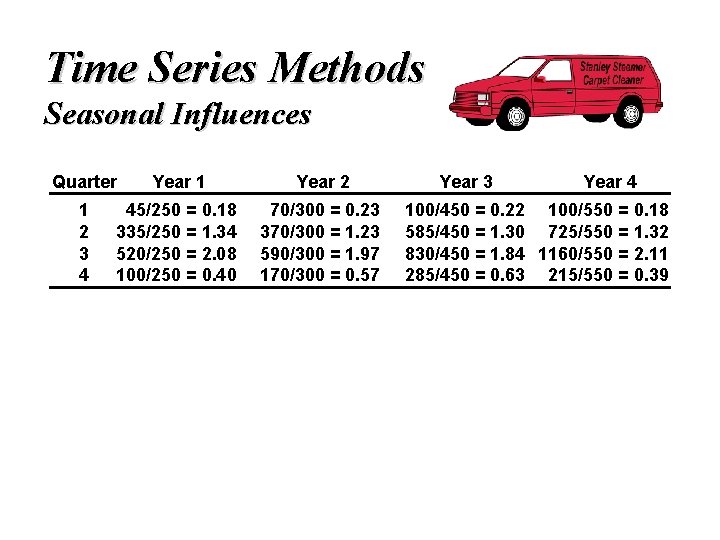
Time Series Methods Seasonal Influences Quarter 1 2 3 4 Year 1 Year 2 45/250 = 0. 18 335/250 = 1. 34 520/250 = 2. 08 100/250 = 0. 40 70/300 = 0. 23 370/300 = 1. 23 590/300 = 1. 97 170/300 = 0. 57 Year 3 Year 4 100/450 = 0. 22 100/550 = 0. 18 585/450 = 1. 30 725/550 = 1. 32 830/450 = 1. 84 1160/550 = 2. 11 285/450 = 0. 63 215/550 = 0. 39

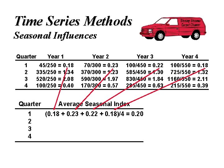
Time Series Methods Seasonal Influences Quarter 1 2 3 4 Year 1 Year 2 45/250 = 0. 18 335/250 = 1. 34 520/250 = 2. 08 100/250 = 0. 40 70/300 = 0. 23 370/300 = 1. 23 590/300 = 1. 97 170/300 = 0. 57 Year 3 Year 4 100/450 = 0. 22 100/550 = 0. 18 585/450 = 1. 30 725/550 = 1. 32 830/450 = 1. 84 1160/550 = 2. 11 285/450 = 0. 63 215/550 = 0. 39 Quarter Average Seasonal Index 1 2 3 4 (0. 18 + 0. 23 + 0. 22 + 0. 18)/4 = 0. 20

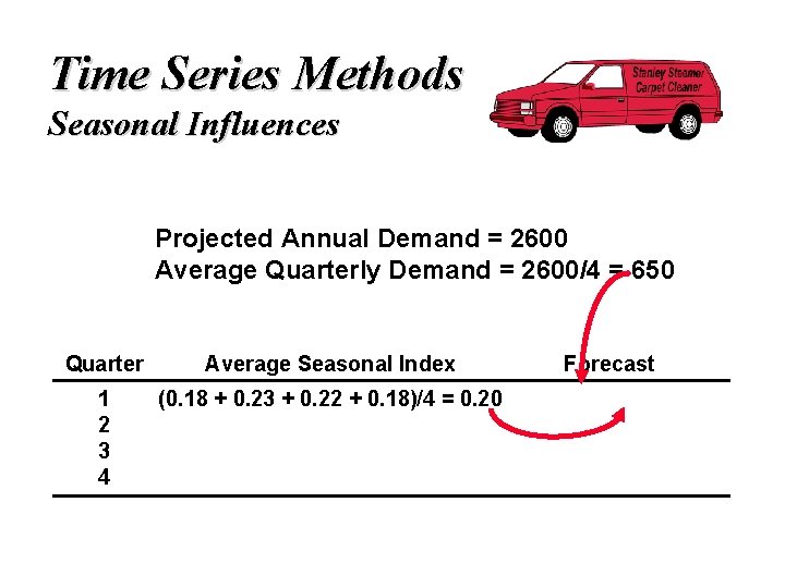
Time Series Methods Seasonal Influences Projected Annual Demand = 2600 Average Quarterly Demand = 2600/4 = 650 Quarter Average Seasonal Index 1 2 3 4 (0. 18 + 0. 23 + 0. 22 + 0. 18)/4 = 0. 20 Forecast

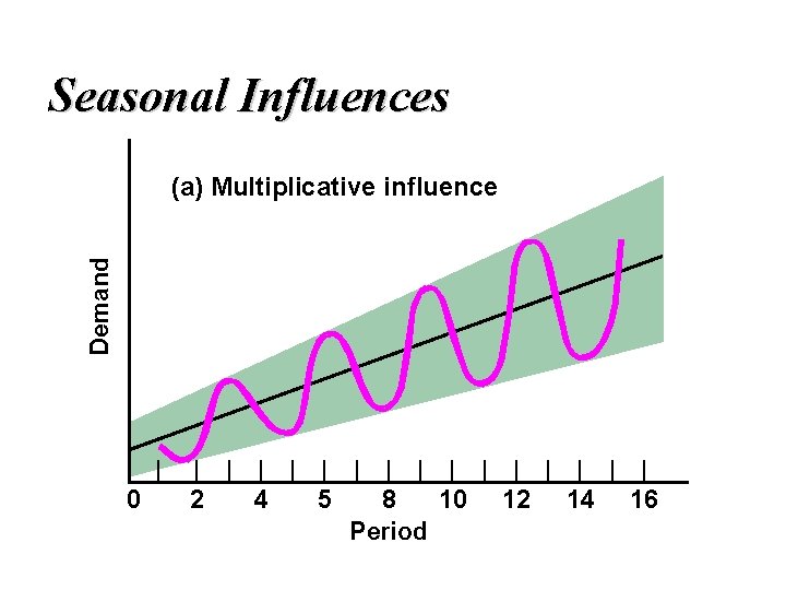
Seasonal Influences Demand (a) Multiplicative influence | 0 | | | | 2 4 5 8 10 12 14 16 Period

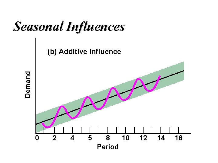
Seasonal Influences Demand (b) Additive influence | 0 | | | | 2 4 5 8 10 12 14 16 Period

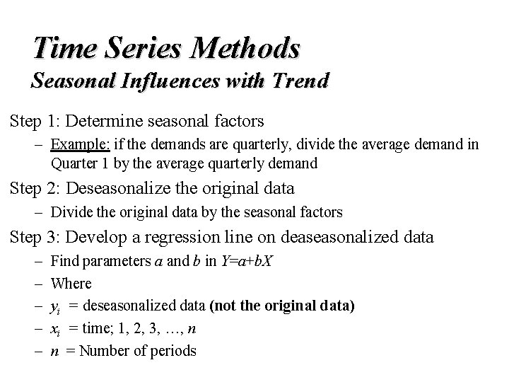
Time Series Methods Seasonal Influences with Trend Step 1: Determine seasonal factors – Example: if the demands are quarterly, divide the average demand in Quarter 1 by the average quarterly demand Step 2: Deseasonalize the original data – Divide the original data by the seasonal factors Step 3: Develop a regression line on deaseasonalized data – – – Find parameters a and b in Y=a+b. X Where yi = deseasonalized data (not the original data) xi = time; 1, 2, 3, …, n n = Number of periods

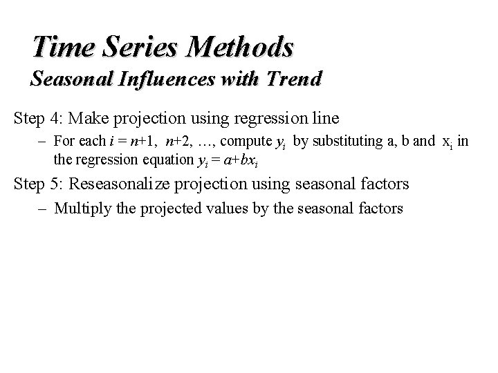
Time Series Methods Seasonal Influences with Trend Step 4: Make projection using regression line – For each i = n+1, n+2, …, compute yi by substituting a, b and xi in the regression equation yi = a+bxi Step 5: Reseasonalize projection using seasonal factors – Multiply the projected values by the seasonal factors

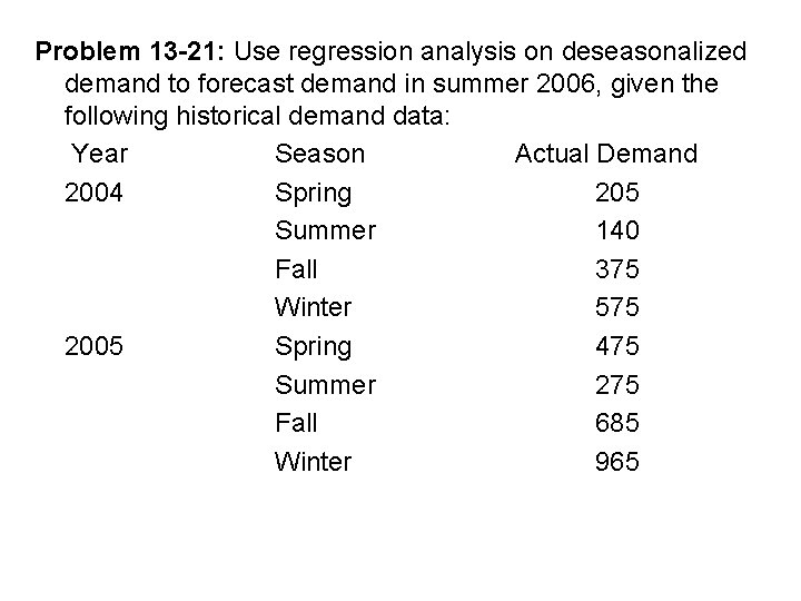
Problem 13 -21: Use regression analysis on deseasonalized demand to forecast demand in summer 2006, given the following historical demand data: Year Season Actual Demand 2004 Spring 205 Summer 140 Fall 375 Winter 575 2005 Spring 475 Summer 275 Fall 685 Winter 965

Reading and Exercises • Chapter 13 pp. 518 -539 • Problems 1, 7, 13, 14, 16