2 0 Linear Timeinvariant Systems 2 1 Discretetime

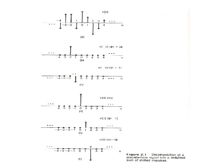
2. 0 Linear Time-invariant Systems 2. 1 Discrete-time Systems: the Convolution Sum l Representing an arbitrary signal as a sequence of unit impulses an unit impulse located at n = k on the index n See Fig. 2. 1, p. 76 of text a special case

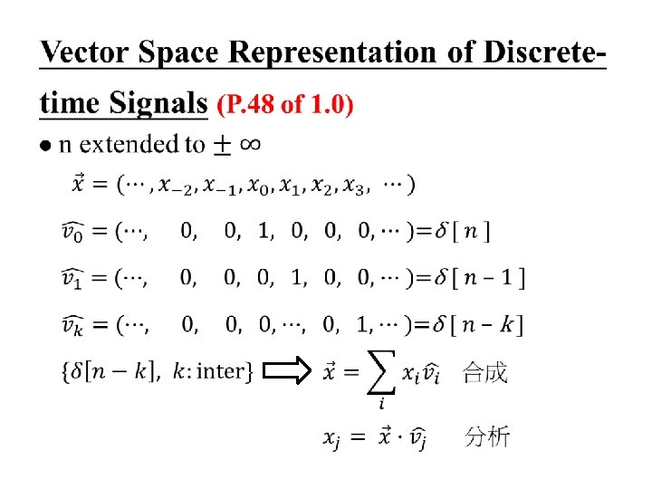
Vector Space Representation of Discretetime Signals (P. 47 of 1. 0) l n-dim

Vector Space Interpretation

Vector Space (P. 30 of 1. 0) 3 -dim Vector Space

N-dim Vector Space (P. 31 of 1. 0) (合成) (分析 )

Vector Space Interpretation

l Representing an arbitrary signal as a sequence of unit impulses (合成) an unit impulse located at n = k on the index n l Sifting property of the unit impulse: looked at on the index k, δ[n-k] is nonzero only at k = n, which “sifts” the value x[n] out of the function x[k]. (分析)

l Defining the output for an unit impulse input as the Unit Impulse Response x[n]= [n] y[n]=h[n]: unit impulse response S 0 n

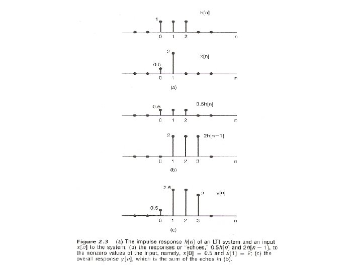
l By Linearity (Superposition Property) – The output for an arbitrary input signal is the superposition of a series of “shifted, scaled unit impulse response” x[k] [n-k] x[k] Convolution Sum See Fig 2. 3, p. 80 of text h[n-k]

Input/Output Relation in Every Dimension

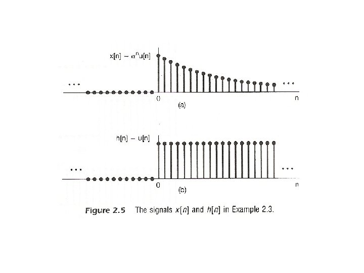
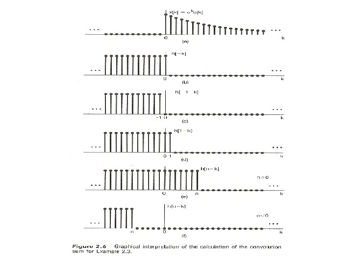
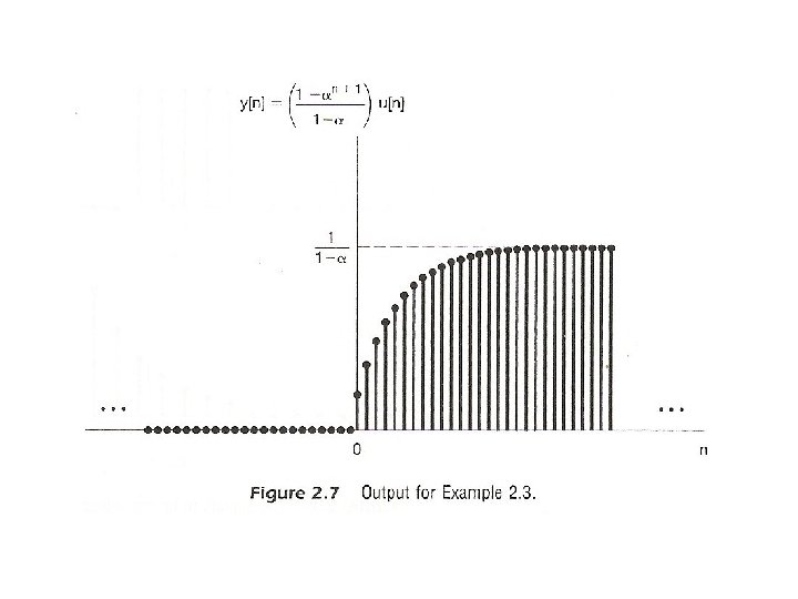
l A Different Way to visualize the convolution sum – looked at on the index k input signal Contribution to the output signal at time n reflected-over version of h[k] located at k = n – on the dummy index k, h[k] is reflected over and shifted to k=n, weighted by x[k] and summed to produce an output sample y[n] at time n See Figs 2. 5, 2. 6, 2. 7, pp. 83 -85 of text

Fig. 2. 6

l A linear time-invariant system is completely characterized by its unit impulse response

Vector Space Concept l Definition of Inner-product – Example – Simple Definition

Inner Product magnitude similarity

Linearity in Inner Product Commutative, Non-degeneracy

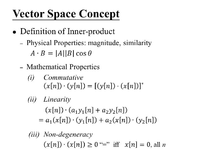
Vector Space Concept l Definition of Inner-product – Physical Properties: magnitude, similarity – For the vector space of signals defined in (N 1, N 2) – Inner-product Space – (N 1, N 2) extended to (-∞, ∞)

Vector Space Concept l Magnitude/Similarity

Vector Space Concept l Orthonormal bases – orthogonal – orthonormal basis any vector (signal) in the vector space can be expanded by the set of orthonormal signals (合成)

System Characterization l Vector Space – Orthonormal bases time-shifted unit impulses, dim = ∞ – A signal expanded by this set of orthonormal basis (合成)

System Characterization l A Different View of the Sifting Property – 3 -dim vector space – Sifting property (分析)

System Characterization l Transformation of Vectors – A System is a Transformation which maps one vector x[n] to another vector y[n] (linear, time-invariant) H[ ]

l Defining the output for an unit impulse input as the Unit Impulse Response (P. 10 of 2. 0) x[n]= [n] y[n]=h[n]: unit impulse response S 0 n

l Rotation as a vector transformation y (1, 0, 0 ) (a, b, c) x Rotation as a vector transformation (1, 0, 0) → (0. 9, 0. 3) (0, 1, 0) → (0. 3, 0. 9, 0. 3) (0, 0, 1) → (0. 3, 0. 9) Rotation plus vector scaling (1, 0, 0, 0, ⋯) → (0. 9, 0. 3, 0. 2, ⋯) (0, 1, 0, 0, ⋯) → ( 0, 0. 9, 0. 3, 0. 2, ⋯) (0, 0, 1, 0, ⋯) → ( 0, 0, 0. 9, 0. 3, 02, ⋯)

Splitting a single basis vector into a few more basis vectors a (a, b, c) b c (1, 0, 0 ) – transforming a single basis vector enough to describe the transformation of any vectors

System Characterization l Transformation of Vectors – unit impulse response is the transformation of δ[n]. A basis vector is transformed to a set of other bases – superposition property for convolution sum

System Characterization l Linear, Time-invariant Transformation of vectors can be expressed by a matrix x y Convolution Sum

System Characterization l Matrix Representation of Convolution Sum example: x[n]=… 0, 0, x 1, x 2, 0, 0, … h[n]=… 0, 0, h 1, h 2, 0, 0, … y[n]=… 0, 0, y 1, y 2, y 3, y 4, 0, 0, …

Matrix Representation 01 2 0 1 2 0 1 2 1 2 3 0 1 2 2 3 4

System Characterization l Matrix Representation of Convolution Sum – each component of the input vector is transformed to a set of other components of the output vector, and all these are superpositioned (superposition property) – each component of the output vector is contributed respectively by the transformed component of each input vector component (reflected, shifted, weighted sum)

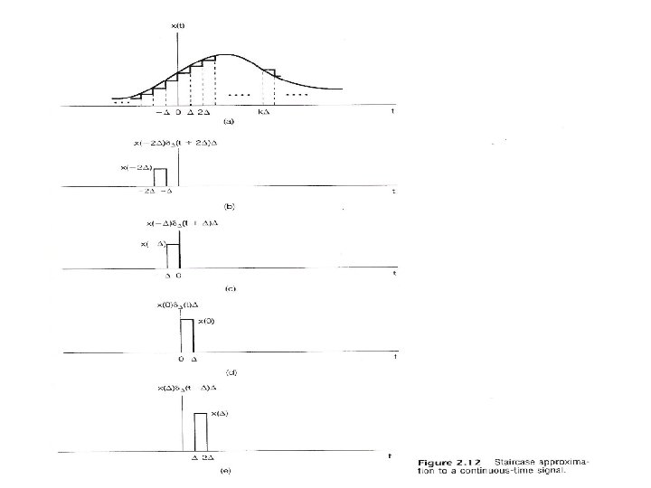
2. 3 Continuous-time System : the Convolution Integral l Representing an arbitrary signal as an integral of impulses See Fig 2. 12 , p. 91 of text an impulse located at t = τ whose value is x(τ) (合成) a special case

Vector Space Interpretation (P. 8 of 2. 0)

Vector Space Representation discrete-time: continuous-

Continuous-time Vector Space

Unit Step 1 0 0 t t – running integral 0 t

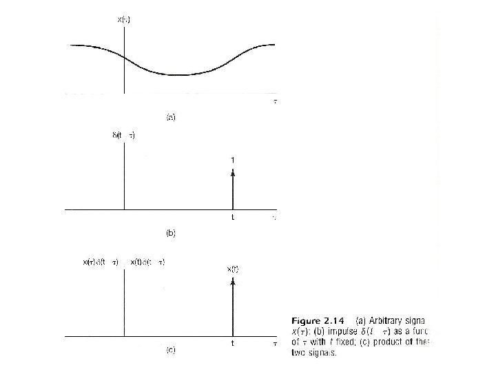
l Representing an arbitrary signal as an integral of impulses – Sifting Property : (分析) Looked at on the index τ, δ(t-τ) located at τ = t shifts the value x(t) out of the function x(τ) See Fig 2. 14 , p. 94 of text

l Defining the output for an unit impulse input as the unit impulse response S 0 t Unit Impulse Response 0 t

l By Linearity (Superposition Property) – The output for an arbitrary input signal is the superposition of a series of “shifted, scaled unit impulse response” Convolution Integral

l Defining the output for an unit impulse input as the Unit Impulse Response (P. 10 of 2. 0) x[n]= [n] y[n]=h[n]: unit impulse response S 0 n

l By Linearity (Superposition Property) (P. 11 of 2. 0) – The output for an arbitrary input signal is the superposition of a series of “shifted, scaled unit impulse response” x[k] [n-k] x[k] Convolution Sum See Fig 2. 3, p. 80 of text h[n-k]

Input/Output Relation in Every Dimension (P. 12 of 2. 0)

Input/Output Relation in Every Dimension 0 0 0

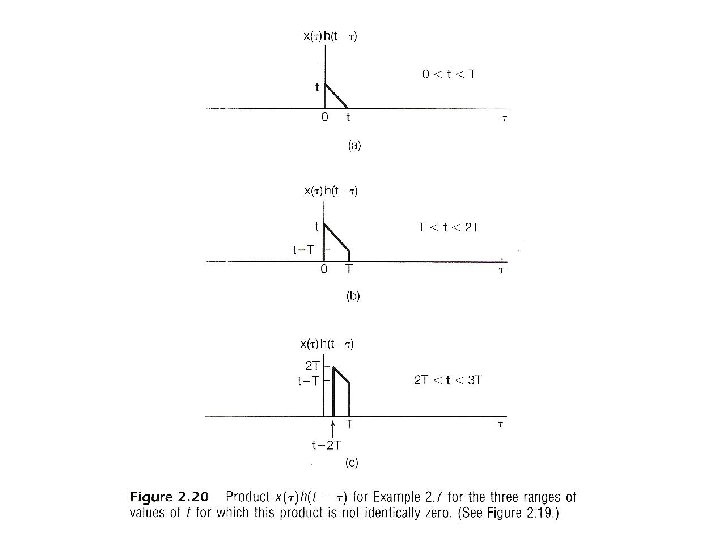
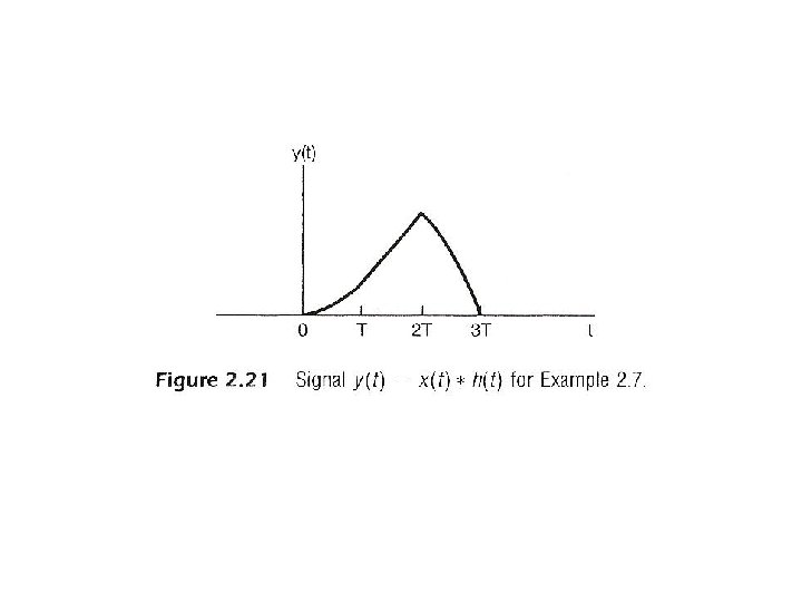
l A Different Way to visualize the convolution integral – Look on the index τ input signal output signal at time t reflected-over version of h(t)located at =t – On the dummy index τ, h(t) is reflected over and shifted to τ = t, weighted by x(t) and integrated to produce the output value at time t, y(t) see Figs. 2. 19, 2. 20, 2. 21, pp. 100 -101 of text l A linear time-invariant system is completely characterized by its unit impulse response

0

2. 4 Properties of Linear Time-invariant Systems l Commutative Property – the role of input signal and unit impulse response is interchangeable, giving the same output signal – In evaluating the convolution sum or integral, the input signal can be reflected over and weighted by the unit impulse response

l Distributive Property additive (linear) property

l Associative Property – Cascade of two systems gives an unit impulse response which is the convolution of the unit impulse responses of the two individual systems – The behavior of a cascade of two systems is independent of the order in which the two systems are cascaded

l Causality – causal if y[n] dose not depend on x[k] for k > n – Causal iff h[n]=0, n < 0

l Causality – continuous-time – Causal iff h(t)=0, t<0

Causality (P. 56 of 1. 0)

Causality & Memory (for future) non-causal memory (for past) non-causal

l Memoryless / with Memory – A linear, time-invariant, causal system is memoryless only if if k=1 further, they are identity systems – sifting property, i. e. , convolution sum (or integral) with an unit impulse function gives the original signal

l Invertibility / Inverse system

l Stability stable if bounded input gives bounded output |x[n]| < B, all n – Stable iff the impulse response is absolutely summable, or absolutely integrable, the necessary condition can be proved

l Unit step response output for an unit step function input Running sum First difference similarly Running integral First derivative

2. 5 Systems Described by Differential/Difference Equations Continuous-time l Differential Equation Specification for Input/Output Relationships – derived by physical phenomena and relationships – very often auxiliary conditions are needed to completely specify the system

Continuous-time l Differential Equation Specification for Input/Output Relationships – the response y(t) to an input x(t) in general consists of two parts: (1) homogeneous solution (natural response): a solution for (2) particular solution: to the complete differential equation

Continuous-time l Initial Rest Condition for Causal Systems – initial conditions

Discrete-time l Difference Equation Specification – derived by sequential behavior of different processes – auxiliary conditions needed – response y(t) consists of two parts (1) homogeneous solution (natural response) for (2) particular solution

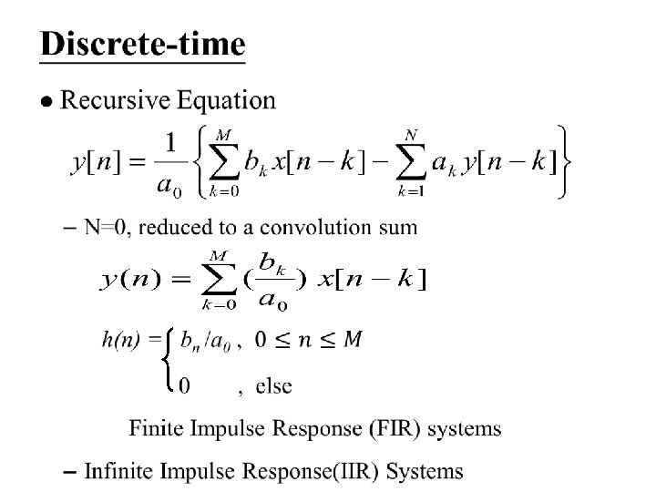
Discrete-time l Initial Rest Condition for Causal Systems l Recursive Equation – output at time n expressed in terms of previous values of input/output

Block Diagram Representation l Elementary Operations x 2[n] x 2(t) x 1[n ] x 1(t) x[n] x(t) x 1[n]+ x 2[n] x 1(t)+ x 2(t) a ax[n] ax(t)

Block Diagram Representation l Elementary Operations x[n] x(t) D x[n-1]

Block Diagram Representation l An Example x[n] b y[n] D -a y[n-1] – Feedback, with memory, initial value of the memory element as the initial condition – Initial rest condition: initial value in the memory element is zero

Block Diagram Representation l Continuous-time Example x(t) y(t)

Block Diagram Representation l Continuous-time Example – Expressed by integrator, assuming initially at rest x(t) b y(t) -a – The integrator represents the memory element

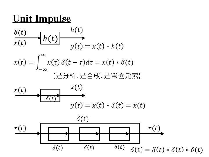
2. 6 The Unit Impulse for Continuous-time Cases Many Different Functions Approaching δ(t) in the Limit l l Sifting Property

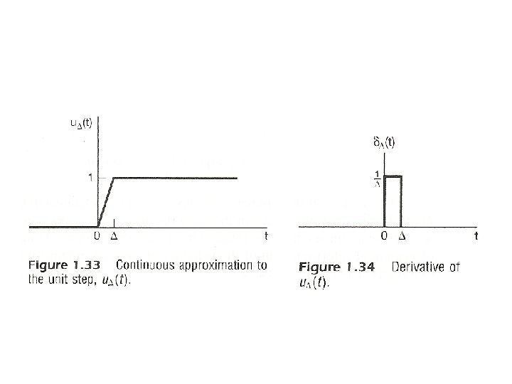
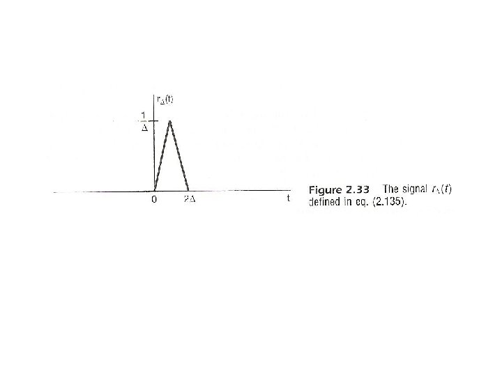
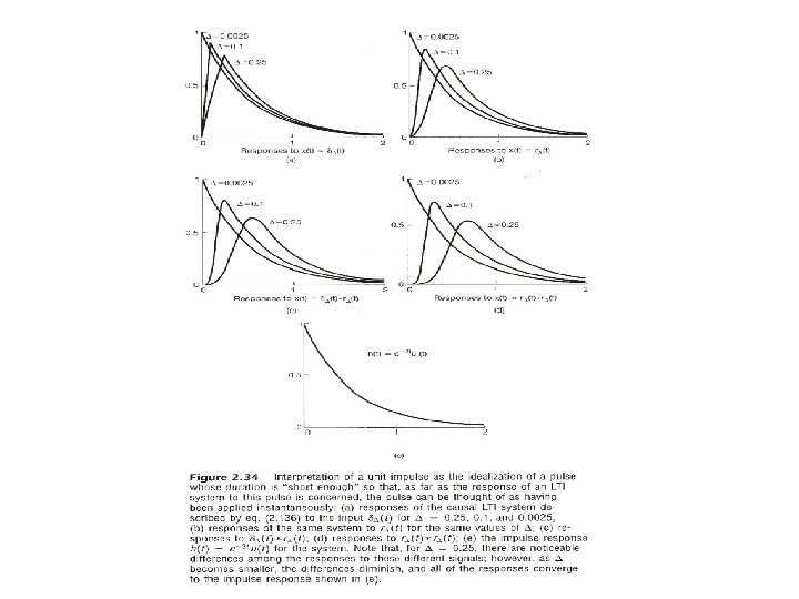
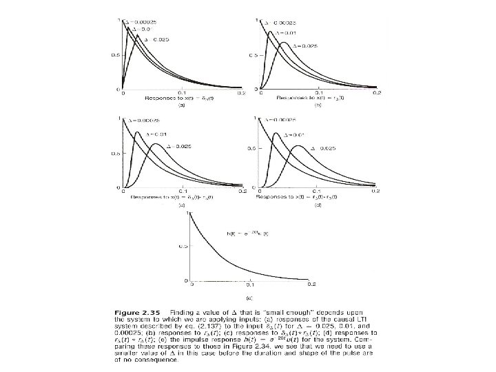
Many Different Functions Approaching δ(t) in the Limit l Let See Fig. 2. 33, p. 128 of text then . .

Many Different Functions Approaching δ(t) in the Limit l Let

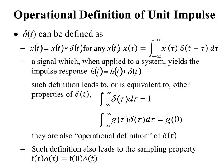
Operational Definition of Unit Impulse l A Function can be defined by – what it is at each value of the independent variable – what it does under some mathematical operation such as an integral or a convolution, or how it behaves with a system, or some mathematical constraints: Singularity Function

Operational Definition of δ(t) 是合成也是分析 是單位元素

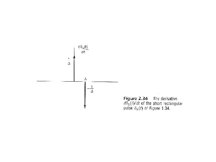
Differentiator, Integrator and Singularity Functions l Differentiator x(t) unit impulse response

See Fig. 2. 36, p. 134 of text

Differentiator, Integrator and Singularity Functions l Cascade of Differentiators k times

Differentiator, Integrator and Singularity Functions l Integrator unit impulse response

Differentiator, Integrator and Singularity Functions l Cascade of Integrators unit ramp function

Differentiator, Integrator and Singularity Functions l Cascade of Integrators k times

Differentiator, Integrator and Singularity Functions l Unified Definition || integrators δ(t) differentiators

Differentiator, Integrator and Singularity Functions l Unified Definition || integrators δ(t) differentiators – operational definitions with singularity functions – manipulate operations efficiently and easily

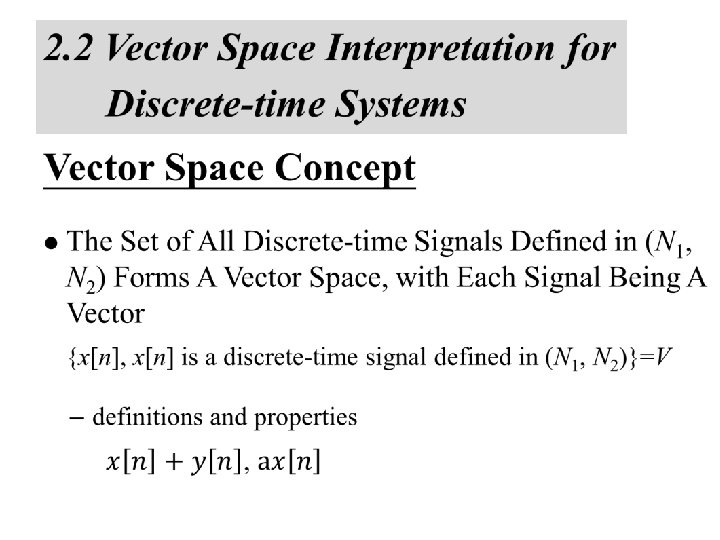
2. 7 Vector Space Interpretation for Continuous-time Systems Vector Space Concept l The Set of All Continuous-time Signals Defined in (t 1, t 2) Forms A Vector Space {x(t), x(t) is a continuous-time signal defined in (t 1, t 2)}=V – definitions and properties

Vector Space Concept l Definition of Inner-product – similar to

Vector Space Concept l Magnitude/Similarity

Inner Product for Continuous-time Signals

Vector Space Concept l Orthonormal Bases – orthogonal – orthonormal

Vector Space Concept – a typical example of orthonormal signal set b: scaling factor – orthonormal basis any vector in the vector space can be expanded by the set of orthonormal signals

Vector Space for Continuous-time Signals l Vector Space l Orthonormal Bases(? ) time-shifted unit impulses, dim=∞ – Inner-product

Vector Space for Continuous-time Signals l Orthonormal Bases(? ) – Inner-product – Not really orthonormal (but are orthogonal), but makes sense under the operational definition

System Characterization l A Signal expanded by unit impulse bases (合成 ) (分析

System Characterization l A System is a Transformation x(t) H y(t) h(t) l Can’t be represented by a matrix due to the discrete property of the matrices, but the concept is the same

Data Transmission “ 0” “ 1” … 1101 … Transmitter 1 1 0 1 channel distortion … 1101 … Decision equalizer front-end filter

Examples • Example 2. 11, p. 110 of text − time shift of signals x(t) h(t) y(t)=x(t-t 0) h(t)= (t-t 0) − convolution of a signal with a shifted impulse is the signal itself but shifted

Examples • Example 2. 12, p. 111 of text − running sum or accumulation x[n] h[n]=u[n] − first difference is the inverse y[n]=x[n]-x[n-1] h 1[n]= [n]- [n-1] − u[n]*{ [n]- [n-1]}=u[n]-u[n-1]= [n]

Examples …

Problem 2. 51(a), p. 154 of text

Problem 2. 64, p. 166 of text • A simplified echo system and its inverse x(t) y(t) …… x(t) T ½ h(t) y(t) (-½) g(t) T

Problem 2. 64, p. 166 of text • A more realistic model x(t) y(t) …… α T h(t) −stability analysis 0<α<1, α>1, x(t) y(t) T (-α) g(t) , stable not integrable, “NOT” stable