Unit II Linear Data Structures Using Sequential Organization

Unit II Linear Data Structures Using Sequential Organization, Linear Data Structure Using Sequential Organization, Array as an Abstract Data Type, Memory Representation and Address Calculation, Inserting an element into an array, Deleting an element, Multidimensional Arrays, Two-dimensional arrays, n- dimensional arrays, Concept of Ordered List, Single Variable Polynomial, Representation using arrays, Polynomial as array of structure, Polynomial addition, Polynomial multiplication, Sparse Matrix, Sparse matrix representation, Sparse matrix addition, Transpose of sparse matrix, String Manipulation Using Array. Case Study- Use of sparse matrix in Social Networks and Maps

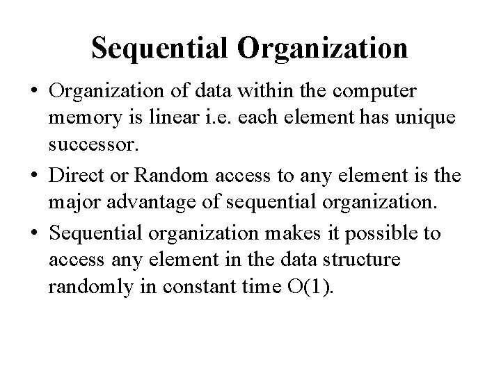
Sequential Organization • Organization of data within the computer memory is linear i. e. each element has unique successor. • Direct or Random access to any element is the major advantage of sequential organization. • Sequential organization makes it possible to access any element in the data structure randomly in constant time O(1).

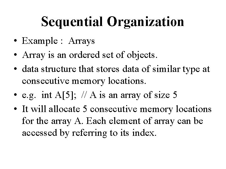
Sequential Organization • Example : Arrays • Array is an ordered set of objects. • data structure that stores data of similar type at consecutive memory locations. • e. g. int A[5]; // A is an array of size 5 • It will allocate 5 consecutive memory locations for the array A. Each element of array can be accessed by referring to its index.

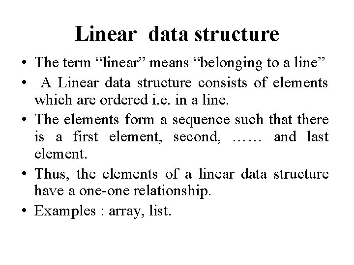
Linear data structure • The term “linear” means “belonging to a line” • A Linear data structure consists of elements which are ordered i. e. in a line. • The elements form a sequence such that there is a first element, second, …… and last element. • Thus, the elements of a linear data structure have a one-one relationship. • Examples : array, list.

Arrays • An array is a finite ordered set of homogenous elements. – Finite : There a specific number of elements in the array. – Ordered : The elements are arranged so that there is a first element, second, and so on. – Homogenous : All the elements are of the same type. • Mathematically, an array can be considered as a set of pairs- (index, value). For each index, there is an associated value. This means that, there is a one-to -one mapping or correspondence between the set of indices and the set of values.

Primitive Operations on Arrays 1. Create : Creating a new array : This needs the information regarding the type of data objects and the number of data objects to be stored. 2. Store(array, index, value) : Store a value at particular position : This needs the name of the array, the position in the array and the value to be stored at that position. 3. Retrieve ( array, index ) : Retrieve a value at a particular position : This operation requires the array name and an index and it returns the corresponding value.

Array as an ADT Objects: A set of pairs <index, value> where for each value of index there is a value from the set item. Index is a finite ordered set of one or more dimensions, for example, {0, … , n-1} for one dimension, {(0, 0), (0, 1), (0, 2), (1, 0), (1, 1), (1, 2), (2, 0), (2, 1), (2, 2)} for two dimensions, etc. Methods: for all A ∈ Array, i ∈ index, x ∈ item, j, size ∈ integer Array Create(j, list) : : = return an array of j dimensions where list is a j-tuple whose kth element is the size of the kth dimension. Items are undefined. Item Retrieve(A, i) : : = if (i ∈ index) return the item associated with index value i in array A else return error Array Store(A, i, x) : : = if (i in index) return an array that is identical to array A except the new pair <i, x> has been inserted else return error

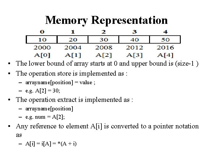
Array Implementation • A single dimension array is created as : – <data type> <array name> [size] ; • Example – int A[5]; • The array is implemented as a constant pointer to the array elements. • The elements are stored in consecutive memory locations. The address of the first element is called the base address.

Memory Representation • The lower bound of array starts at 0 and upper bound is (size-1 ) • The operation store is implemented as : – arrayname[position] = value ; – e. g. A[2] = 30; • The operation extract is implemented as : – arrayname[position] – e. g. num = A[2]; • Any reference to element A[i] is converted to a pointer notation as – A[i] = i[A] = *(A + i)

Address Calculation • Address of A[i] = Base Address + i * element size • E. g. • Address of A[3] = 2000 + 3 * sizeof(int) = 2000 + 3 * 4 = 2012

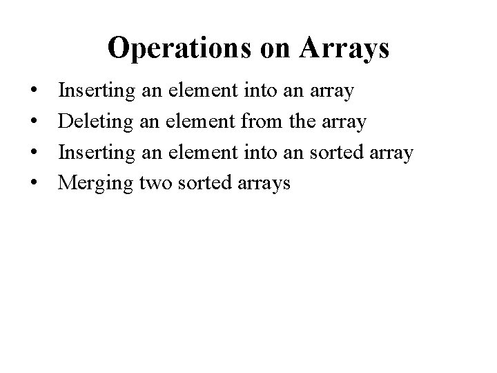
Operations on Arrays • • Inserting an element into an array Deleting an element from the array Inserting an element into an sorted array Merging two sorted arrays

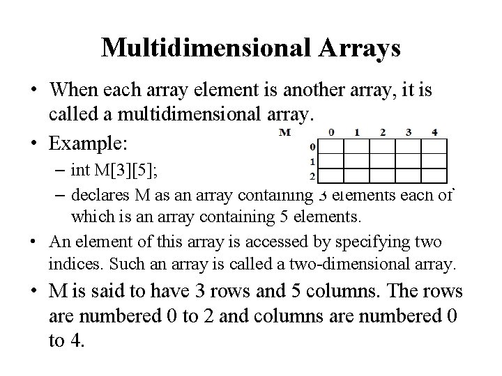
Multidimensional Arrays • When each array element is another array, it is called a multidimensional array. • Example: – int M[3][5]; – declares M as an array containing 3 elements each of which is an array containing 5 elements. • An element of this array is accessed by specifying two indices. Such an array is called a two-dimensional array. • M is said to have 3 rows and 5 columns. The rows are numbered 0 to 2 and columns are numbered 0 to 4.

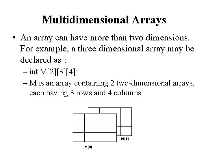
Multidimensional Arrays • An array can have more than two dimensions. For example, a three dimensional array may be declared as : – int M[2][3][4]; – M is an array containing 2 two-dimensional arrays, each having 3 rows and 4 columns.

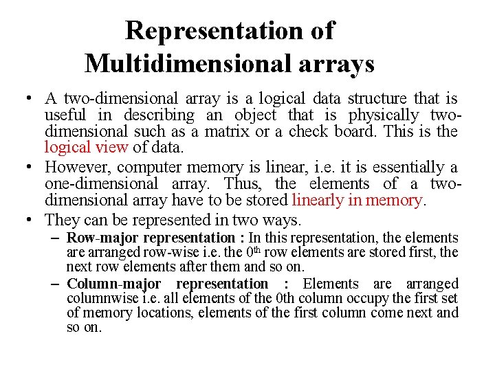
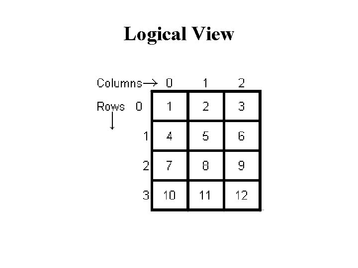
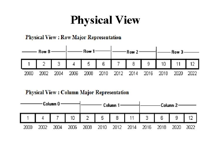
Representation of Multidimensional arrays • A two-dimensional array is a logical data structure that is useful in describing an object that is physically twodimensional such as a matrix or a check board. This is the logical view of data. • However, computer memory is linear, i. e. it is essentially a one-dimensional array. Thus, the elements of a twodimensional array have to be stored linearly in memory. • They can be represented in two ways. – Row-major representation : In this representation, the elements are arranged row-wise i. e. the 0 th row elements are stored first, the next row elements after them and so on. – Column-major representation : Elements are arranged columnwise i. e. all elements of the 0 th column occupy the first set of memory locations, elements of the first column come next and so on.

Logical View

Physical View

Address Calculation For an array int M[R][C]; where R = number of rows and C = number of columns , the location of an element M[i][j] in the array can be calculated as : Address of M[i][j] = Base Address + i * C * Element size + j * Element size = Base Address + ( i * C + j ) * Element size Example : Address of M[1][2] = 2000 + ( 1 * 3 + 2 ) * sizeof (int) = 2000 + 5 * 2 = 2010

Address Calculation For an array int M[R][C]; where R = number of rows and C = number of columns , the location of an element M[i][j] in the array can be calculated as : Address of M[i][j] = Base Address + j * R * Element size + i * Element size = Base Address + ( j * R + i ) * Element size Example : Address of M[1][2] = 2000 + ( 2 * 4 + 1 ) * sizeof (int) = 2000 + 9 * 2 = 2018

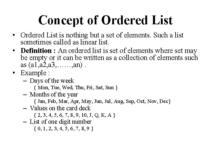
Concept of Ordered List • Ordered List is nothing but a set of elements. Such a list sometimes called as linear list. • Definition : An ordered list is set of elements where set may be empty or it can be written as a collection of elements such as (a 1, a 2, a 3, ……, an). • Example : – Days of the week { Mon, Tue, Wed, Thu, Fri, Sat, Sun } – Months of the year { Jan, Feb, Mar, Apr, May, Jun, Jul, Aug, Sep, Oct, Nov, Dec} – Values on the card deck { 2, 3, 4, 5, 6, 7, 8, 9, 10, J, Q, K, A } – List of one digit number { 0, 1, 2, 3, 4, 5, 6, 7, 8, 9 }

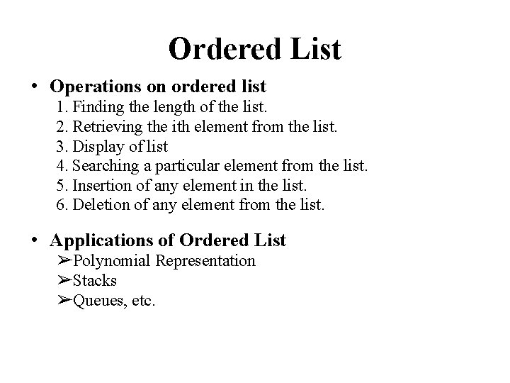
Ordered List • Operations on ordered list 1. Finding the length of the list. 2. Retrieving the ith element from the list. 3. Display of list 4. Searching a particular element from the list. 5. Insertion of any element in the list. 6. Deletion of any element from the list. • Applications of Ordered List ➢Polynomial Representation ➢Stacks ➢Queues, etc.

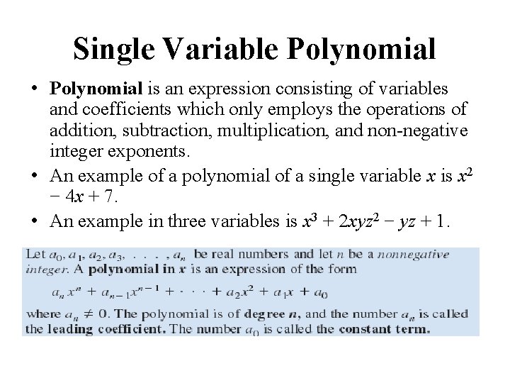
Single Variable Polynomial • Polynomial is an expression consisting of variables and coefficients which only employs the operations of addition, subtraction, multiplication, and non-negative integer exponents. • An example of a polynomial of a single variable x is x 2 − 4 x + 7. • An example in three variables is x 3 + 2 xyz 2 − yz + 1.

Polynomials Use • Polynomials appear in a wide variety of areas of mathematics and science. • Used to form polynomial equations, which encode a wide range of problems, from elementary word problems to complicated problems in the sciences; • Used to define polynomial functions, which appear in settings ranging from basic chemistry and physics to economics and social science; • Used in calculus and numerical analysis to approximate other functions. • In advanced mathematics, polynomials are used to construct polynomial rings and algebraic varieties, central concepts in algebra and algebraic geometry.

Representation using arrays • One Dimensional Array • Two Dimensional Array • Array of Structures

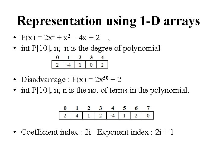
Representation using 1 -D arrays • F(x) = 2 x 4 + x 2 – 4 x + 2 , • int P[10], n; n is the degree of polynomial • Disadvantage : F(x) = 2 x 50 + 2 • int P[10], n; n is the no. of terms in the polynomial. • Coefficient index : 2 i Exponent index : 2 i + 1

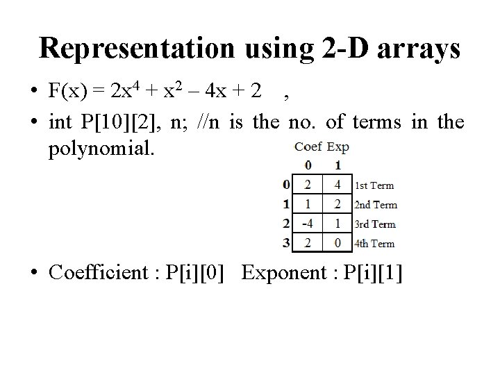
Representation using 2 -D arrays • F(x) = 2 x 4 + x 2 – 4 x + 2 , • int P[10][2], n; //n is the no. of terms in the polynomial. • Coefficient : P[i][0] Exponent : P[i][1]

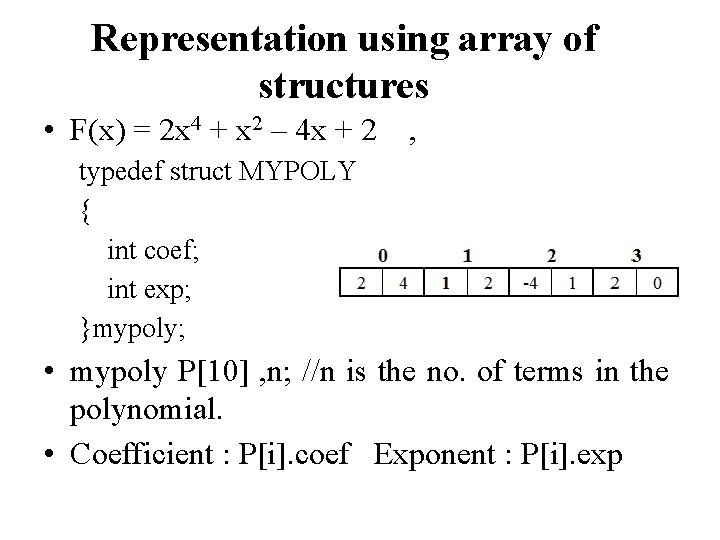
Representation using array of structures • F(x) = 2 x 4 + x 2 – 4 x + 2 , typedef struct MYPOLY { int coef; int exp; }mypoly; • mypoly P[10] , n; //n is the no. of terms in the polynomial. • Coefficient : P[i]. coef Exponent : P[i]. exp

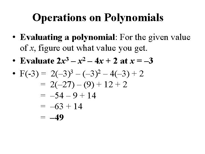
Operations on Polynomials • Evaluating a polynomial: For the given value of x, figure out what value you get. • Evaluate 2 x 3 – x 2 – 4 x + 2 at x = – 3 • F(-3) = 2(– 3)3 – (– 3)2 – 4(– 3) + 2 = 2(– 27) – (9) + 12 + 2 = – 54 – 9 + 14 = – 63 + 14 = – 49

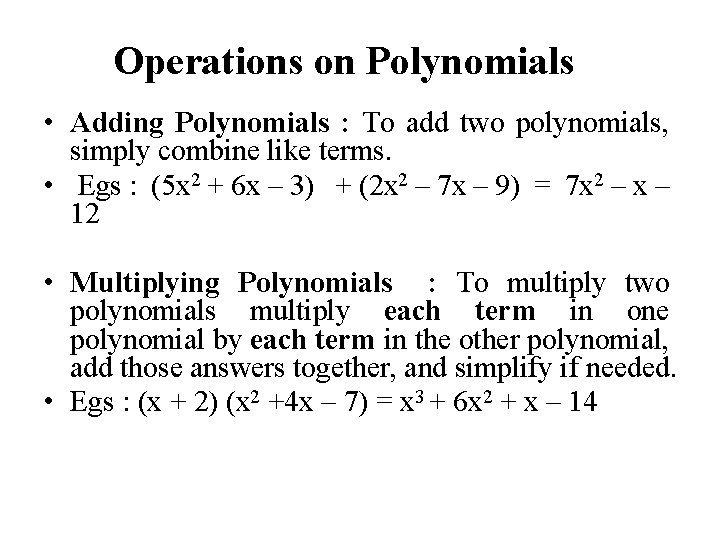
Operations on Polynomials • Adding Polynomials : To add two polynomials, simply combine like terms. • Egs : (5 x 2 + 6 x – 3) + (2 x 2 – 7 x – 9) = 7 x 2 – x – 12 • Multiplying Polynomials : To multiply two polynomials multiply each term in one polynomial by each term in the other polynomial, add those answers together, and simplify if needed. • Egs : (x + 2) (x 2 +4 x – 7) = x 3 + 6 x 2 + x – 14

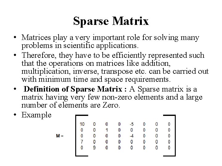
Sparse Matrix • Matrices play a very important role for solving many problems in scientific applications. • Therefore, they have to be efficiently represented such that the operations on matrices like addition, multiplication, inverse, transpose etc. can be carried out with minimum time and space requirements. • Definition of Sparse Matrix : A Sparse matrix is a matrix having very few non-zero elements and a large number of elements are Zero. • Example :

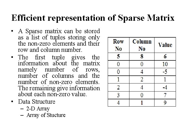
Efficient representation of Sparse Matrix • A Sparse matrix can be stored as a list of tuples storing only the non-zero elements and their row and column number. • The first tuple gives the information about the matrix namely number of rows, number of columns and the number of non-zero elements. The remaining give information about each non-zero value. • Data Structure – 2 -D Array – Array of Stucture

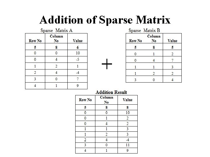
Addition of Sparse Matrix

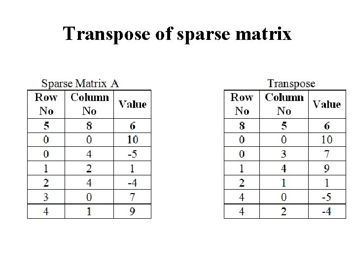
Transpose of sparse matrix

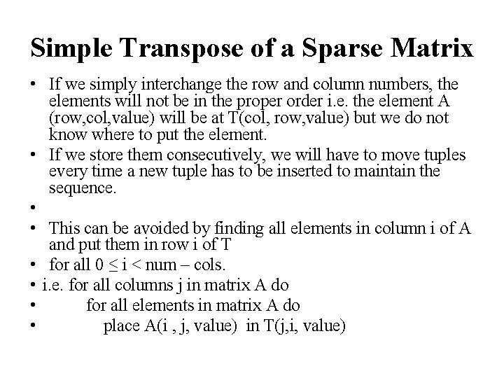
Simple Transpose of a Sparse Matrix • If we simply interchange the row and column numbers, the elements will not be in the proper order i. e. the element A (row, col, value) will be at T(col, row, value) but we do not know where to put the element. • If we store them consecutively, we will have to move tuples every time a new tuple has to be inserted to maintain the sequence. • • This can be avoided by finding all elements in column i of A and put them in row i of T • for all 0 ≤ i < num – cols. • i. e. for all columns j in matrix A do • for all elements in matrix A do • place A(i , j, value) in T(j, i, value)

Simple Transpose of a Sparse Matrix void Simple_transpose_sparse_matrix(struct sparse s[], struct sparse t[]) { int i, j, k=1; for(i=0; i<s[0]. col; i++) { for(j=1; j<=s[0]. val; j++) { if(s[j]. col == i) { t[k]. row = s[j]. col; t[k]. col = s[j]. row; t[k]. val = s[j]. val; k++; } } t[0]. row = s[0]. col; t[0]. col = s[0]. row; t[0]. val = s[0]. val; }

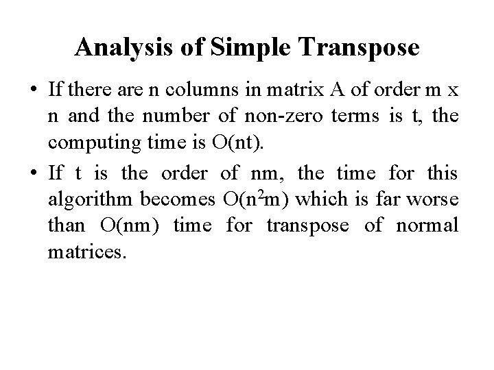
Analysis of Simple Transpose • If there are n columns in matrix A of order m x n and the number of non-zero terms is t, the computing time is O(nt). • If t is the order of nm, the time for this algorithm becomes O(n 2 m) which is far worse than O(nm) time for transpose of normal matrices.

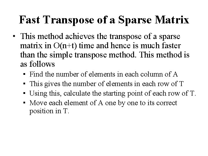
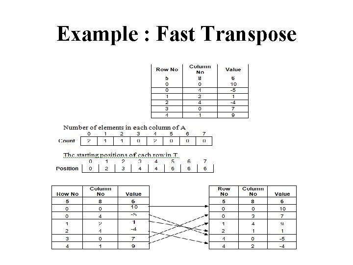
Fast Transpose of a Sparse Matrix • This method achieves the transpose of a sparse matrix in O(n+t) time and hence is much faster than the simple transpose method. This method is as follows ▪ ▪ Find the number of elements in each column of A This gives the number of elements in each row of T Using this, calculate the starting point of each row of T. Move each element of A one by one to its correct position in T.

Example : Fast Transpose

Fast Transpose of a Sparse Matrix void Fast_transpose_sparse_matrix(struct sparse s[], struct sparse t[]) { static int pos[15], term[15]; t[0]. row = s[0]. col; t[0]. col = s[0]. row; t[0]. val = s[0]. val; for(i=1; i<=s[0]. val; i++) term[s[i]. col]++; pos[0] = 1; for(i=1; i<s[0]. col; i++) pos[i] = pos[i-1] + term[i-1]; for(i=1; i<=s[0]. val; i++) { t[pos[s[i]. col]]. row = s[i]. col; t[pos[s[i]. col]]. col = s[i]. row; t[pos[s[i]. col]]. val = s[i]. val; pos[s[i]. col]++; } }

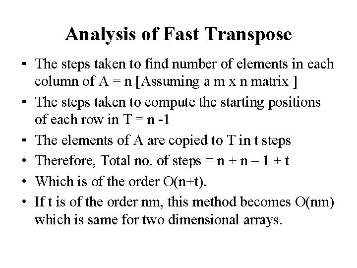
Analysis of Fast Transpose ▪ The steps taken to find number of elements in each column of A = n [Assuming a m x n matrix ] ▪ The steps taken to compute the starting positions of each row in T = n -1 ▪ The elements of A are copied to T in t steps • Therefore, Total no. of steps = n + n – 1 + t • Which is of the order O(n+t). • If t is of the order nm, this method becomes O(nm) which is same for two dimensional arrays.

Case Study ▪ Application of Sparse Matrix ▪ Social Networks ▪ Maps

String Manipulation Using Array ▪ A string is a character array terminated by a null character () ▪ Operations on Strings – String Length – String Copy – String Concatenation – String Reverse – String Compare – Substring, etc

Thank you