Section 6 6 Graphing Linear Inequalities in Two

Section 6 -6 Graphing Linear Inequalities in Two Variables

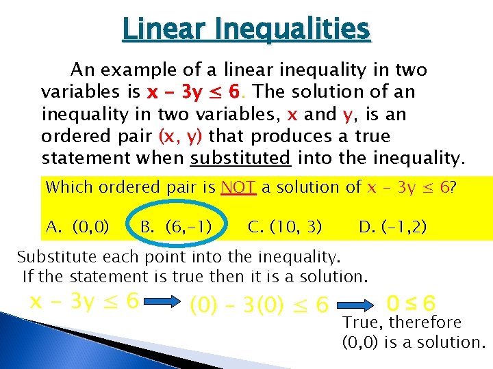
Linear Inequalities An example of a linear inequality in two variables is x - 3 y ≤ 6. The solution of an inequality in two variables, x and y, is an ordered pair (x, y) that produces a true statement when substituted into the inequality. Which ordered pair is NOT a solution of x - 3 y ≤ 6? A. (0, 0) B. (6, -1) C. (10, 3) D. (-1, 2) Substitute each point into the inequality. If the statement is true then it is a solution. x - 3 y ≤ 6 (0) – 3(0) ≤ 6 0≤ 6 True, therefore (0, 0) is a solution.

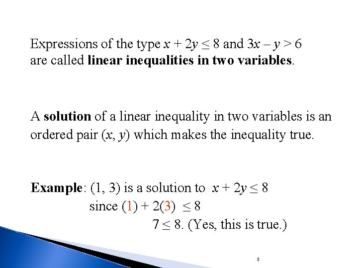
Expressions of the type x + 2 y ≤ 8 and 3 x – y > 6 are called linear inequalities in two variables. A solution of a linear inequality in two variables is an ordered pair (x, y) which makes the inequality true. Example: (1, 3) is a solution to x + 2 y ≤ 8 since (1) + 2(3) ≤ 8 7 ≤ 8. (Yes, this is true. ) 3

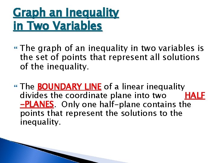
Graph an Inequality in Two Variables The graph of an inequality in two variables is the set of points that represent all solutions of the inequality. The BOUNDARY LINE of a linear inequality divides the coordinate plane into two HALF -PLANES. Only one half-plane contains the points that represent the solutions to the inequality.

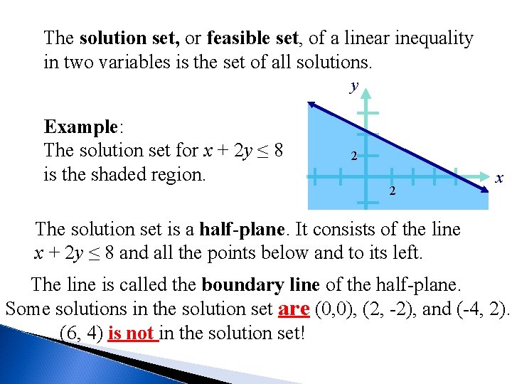
The solution set, or feasible set, of a linear inequality in two variables is the set of all solutions. y Example: The solution set for x + 2 y ≤ 8 is the shaded region. 2 2 x The solution set is a half-plane. It consists of the line x + 2 y ≤ 8 and all the points below and to its left. The line is called the boundary line of the half-plane. Some solutions in the solution set are (0, 0), (2, -2), and (-4, 2). (6, 4) is not in the solution set!

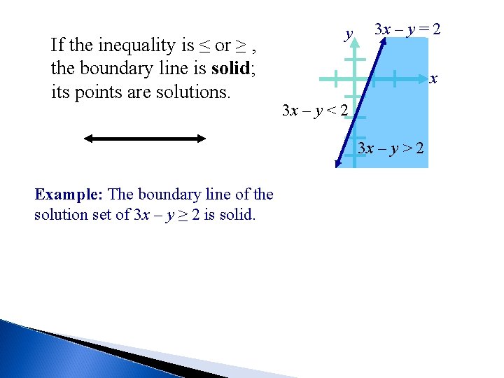
If the inequality is ≤ or ≥ , the boundary line is solid; its points are solutions. y 3 x – y = 2 x 3 x – y < 2 3 x – y > 2 Example: The boundary line of the solution set of 3 x – y ≥ 2 is solid.

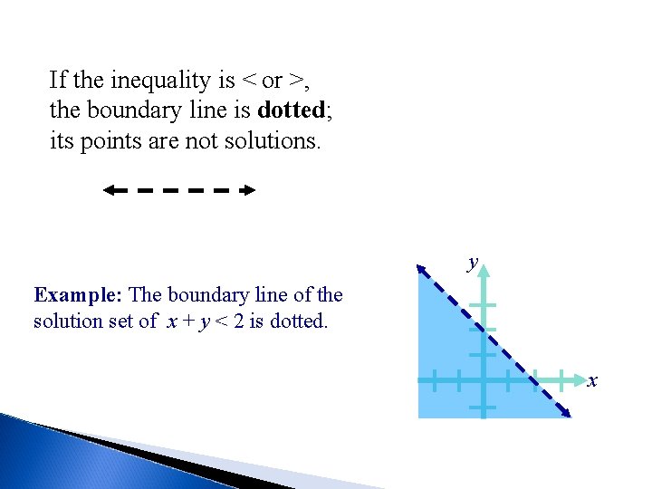
If the inequality is < or >, the boundary line is dotted; its points are not solutions. y Example: The boundary line of the solution set of x + y < 2 is dotted. x

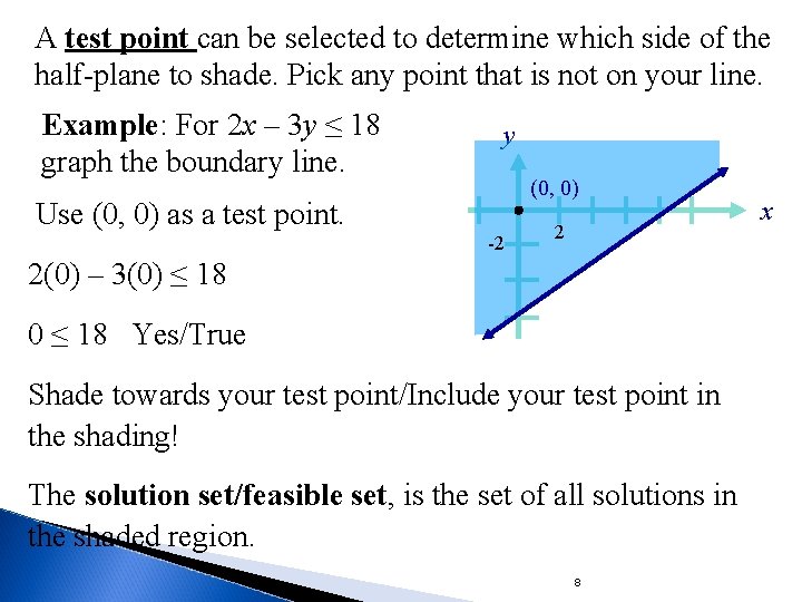
A test point can be selected to determine which side of the half-plane to shade. Pick any point that is not on your line. Example: For 2 x – 3 y ≤ 18 graph the boundary line. y (0, 0) Use (0, 0) as a test point. -2 2 2(0) – 3(0) ≤ 18 0 ≤ 18 Yes/True Shade towards your test point/Include your test point in the shading! The solution set/feasible set, is the set of all solutions in the shaded region. 8 x

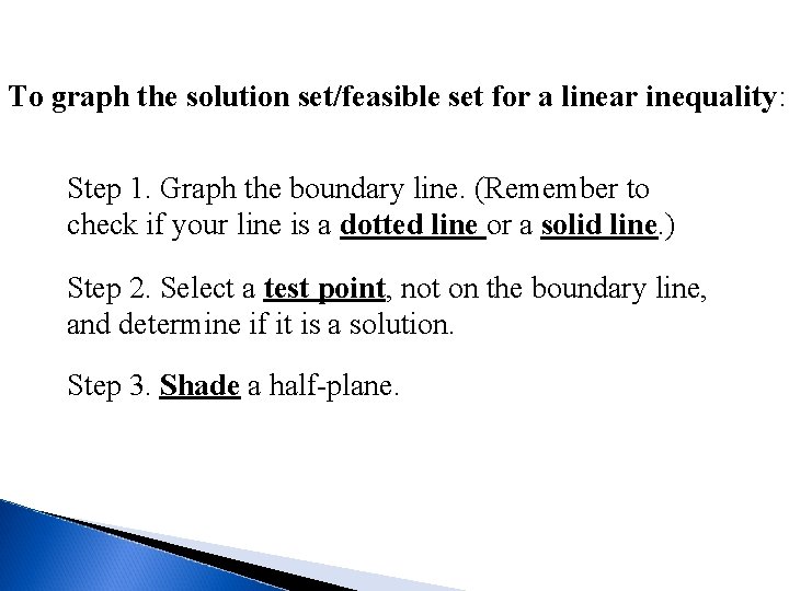
To graph the solution set/feasible set for a linear inequality: Step 1. Graph the boundary line. (Remember to check if your line is a dotted line or a solid line. ) Step 2. Select a test point, not on the boundary line, and determine if it is a solution. Step 3. Shade a half-plane.

Example: Graph the solution set for x – y > 2. Step 1. ) Graph the boundary line x – y = 2 as a dotted line. Step 2. ) Select a test point not on the line, say (0, 0) x–y>2 (2, 0) (0) – (0) > 2 x (0, -2) 0 > 2 No/False! Step 3. ) Since this is a not a solution, shade in the half-plane not containing (0, 0). Or, shade away from your test point. The solution set/feasible set, is the set of all solutions in the shaded region. 10

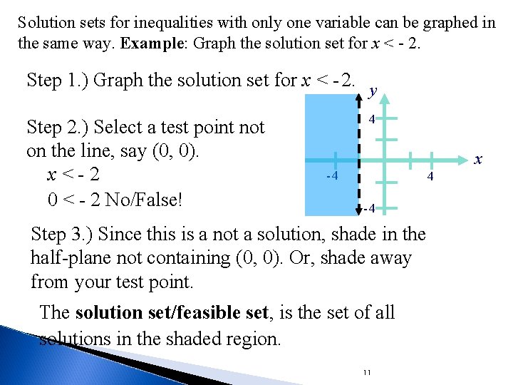
Solution sets for inequalities with only one variable can be graphed in the same way. Example: Graph the solution set for x < - 2. Step 1. ) Graph the solution set for x < - 2. y Step 2. ) Select a test point not on the line, say (0, 0). x<-2 0 < - 2 No/False! 4 x -4 4 -4 Step 3. ) Since this is a not a solution, shade in the half-plane not containing (0, 0). Or, shade away from your test point. The solution set/feasible set, is the set of all solutions in the shaded region. 11

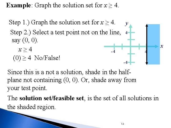
Example: Graph the solution set for x ≥ 4. Step 1. ) Graph the solution set for x ≥ 4. y Step 2. ) Select a test point not on the line, 4 say (0, 0). x≥ 4 -4 (0) ≥ 4 No/False! x 4 -4 Since this is a not a solution, shade in the halfplane not containing (0, 0). Or, shade away from your test point. The solution set/feasible set, is the set of all solutions in the shaded region. 12

Graph an Inequality Graph the inequality STEP 1 Graph the equation STEP 2 Test (0, 0) in the original inequality. y > 4 x - 3. STEP 3 Shade the half-plane that contains the point (0, 0), because (0, 0) is a solution to the inequality.

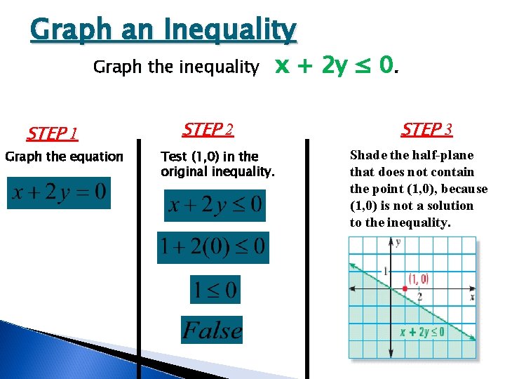
Graph an Inequality Graph the inequality STEP 1 Graph the equation STEP 2 Test (1, 0) in the original inequality. x + 2 y ≤ 0. STEP 3 Shade the half-plane that does not contain the point (1, 0), because (1, 0) is not a solution to the inequality.

Graph an Inequality Graph the inequality STEP 1 Graph the equation STEP 2 Test (0, 0) in the original inequality. -1 ≤ x + y. STEP 3 Shade the half-plane that contains the point (0, 0), because (0, 0) is a solution to the inequality.

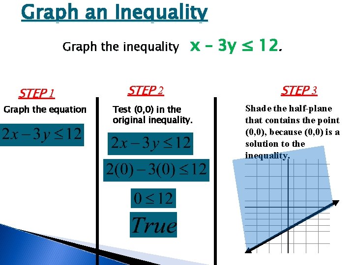
Graph an Inequality Graph the inequality STEP 1 Graph the equation x – 3 y ≤ 12. STEP 2 Test (0, 0) in the original inequality. STEP 3 Shade the half-plane that contains the point (0, 0), because (0, 0) is a solution to the inequality.

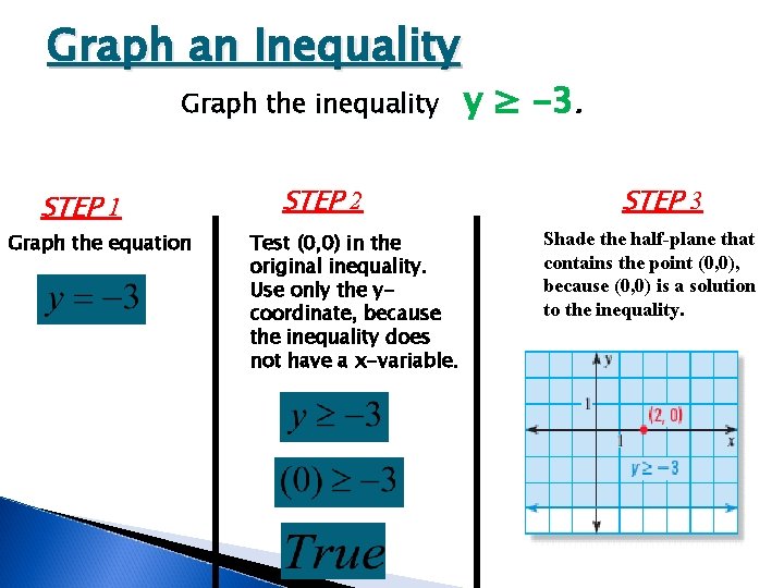
Graph an Inequality Graph the inequality STEP 1 Graph the equation STEP 2 Test (0, 0) in the original inequality. Use only the ycoordinate, because the inequality does not have a x-variable. y ≥ -3. STEP 3 Shade the half-plane that contains the point (0, 0), because (0, 0) is a solution to the inequality.

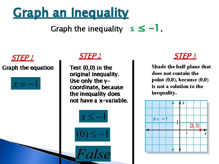
Graph an Inequality Graph the inequality STEP 1 Graph the equation STEP 2 Test (0, 0) in the original inequality. Use only the ycoordinate, because the inequality does not have a x-variable. x ≤ -1. STEP 3 Shade the half-plane that does not contain the point (0, 0), because (0, 0) is not a solution to the inequality.

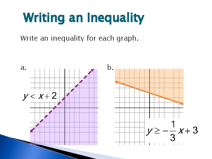
Writing an Inequality Write an inequality for each graph. a. b.

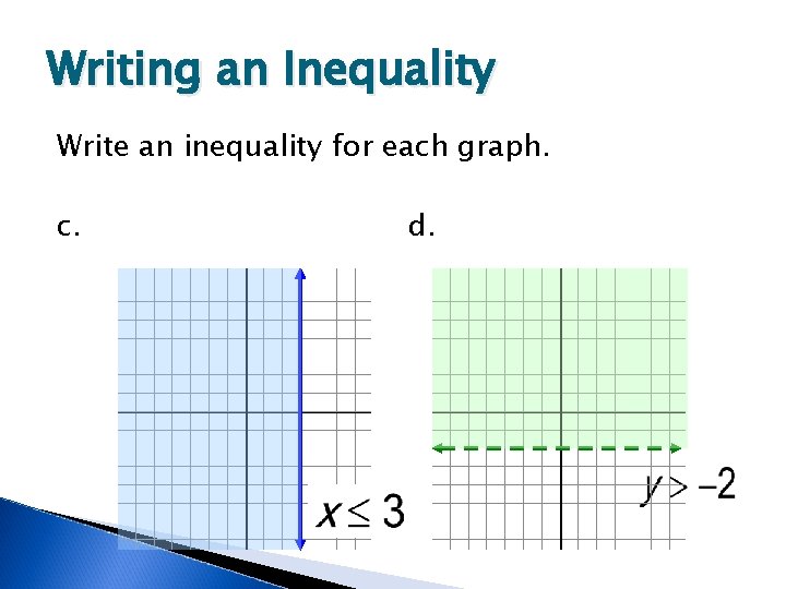
Writing an Inequality Write an inequality for each graph. c. d.

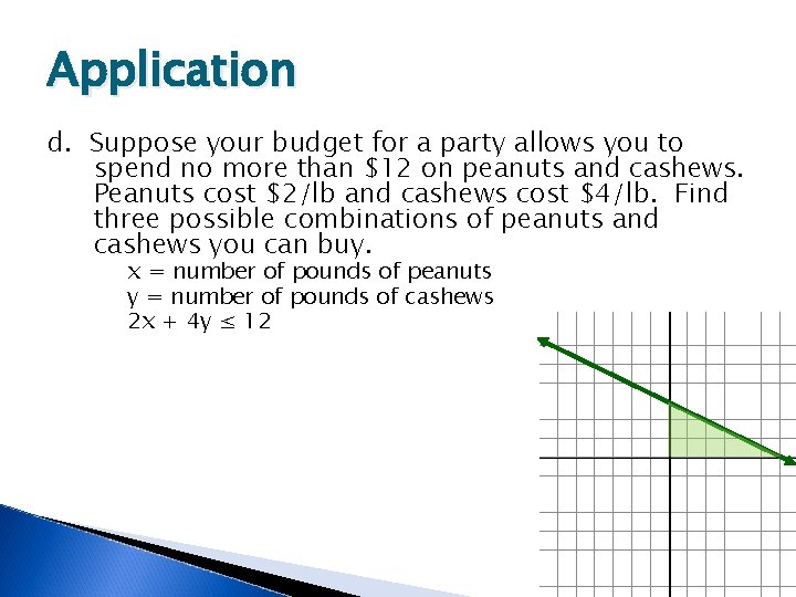
Application d. Suppose your budget for a party allows you to spend no more than $12 on peanuts and cashews. Peanuts cost $2/lb and cashews cost $4/lb. Find three possible combinations of peanuts and cashews you can buy. x = number of pounds of peanuts y = number of pounds of cashews 2 x + 4 y ≤ 12

Assignment Study Guide 6 -6 (In-Class) 6 -5 Skills Practice Worksheet and 6 -6 Skills Practice Worksheet 6 -5/6 -6 Quiz on Thursday 3 -5 -15 Unit 5 (aka chapter 6) Test on Wednestday 3 -11 -15

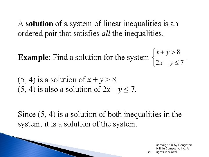
A solution of a system of linear inequalities is an ordered pair that satisfies all the inequalities. Example: Find a solution for the system . (5, 4) is a solution of x + y > 8. (5, 4) is also a solution of 2 x – y ≤ 7. Since (5, 4) is a solution of both inequalities in the system, it is a solution of the system. 23 Copyright © by Houghton Mifflin Company, Inc. All rights reserved.

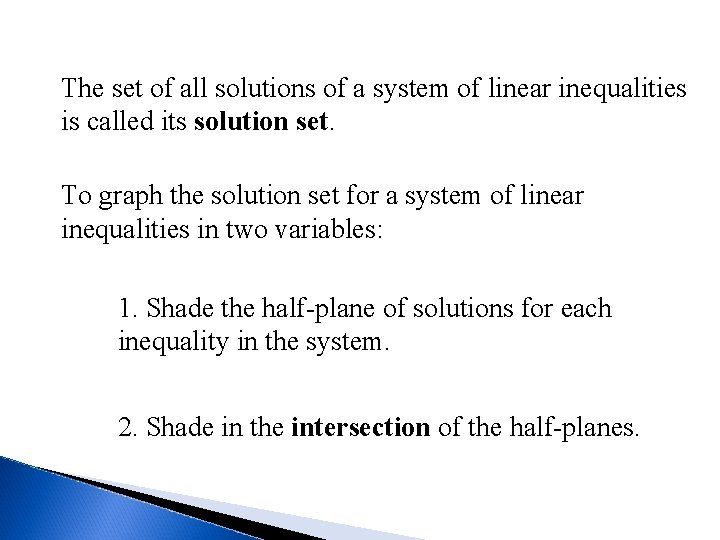
The set of all solutions of a system of linear inequalities is called its solution set. To graph the solution set for a system of linear inequalities in two variables: 1. Shade the half-plane of solutions for each inequality in the system. 2. Shade in the intersection of the half-planes.

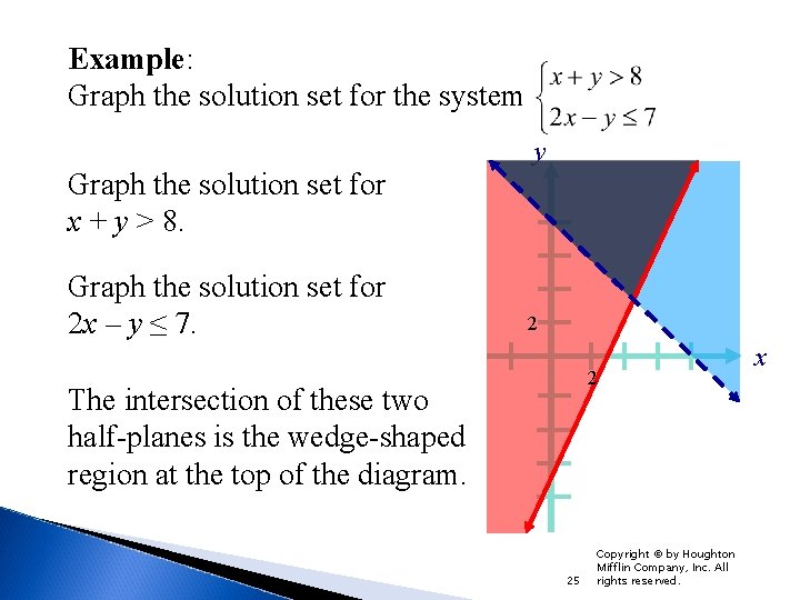
Example: Graph the solution set for the system y Graph the solution set for x + y > 8. Graph the solution set for 2 x – y ≤ 7. 2 2 The intersection of these two half-planes is the wedge-shaped region at the top of the diagram. 25 Copyright © by Houghton Mifflin Company, Inc. All rights reserved. x

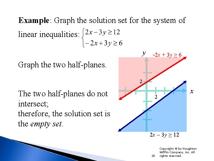
Example: Graph the solution set for the system of linear inequalities: y -2 x + 3 y ≥ 6 Graph the two half-planes. 2 The two half-planes do not intersect; therefore, the solution set is the empty set. x 2 2 x – 3 y ≥ 12 26 Copyright © by Houghton Mifflin Company, Inc. All rights reserved.

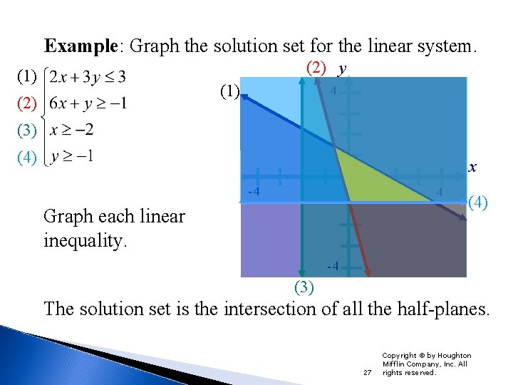
Example: Graph the solution set for the linear system. (2) y (1) (2) 4 (3) (4) x -4 4 Graph each linear inequality. (4) -4 (3) The solution set is the intersection of all the half-planes. 27 Copyright © by Houghton Mifflin Company, Inc. All rights reserved.