2 Linear TimeInvariant Systems 2 1 Discretetime LTI

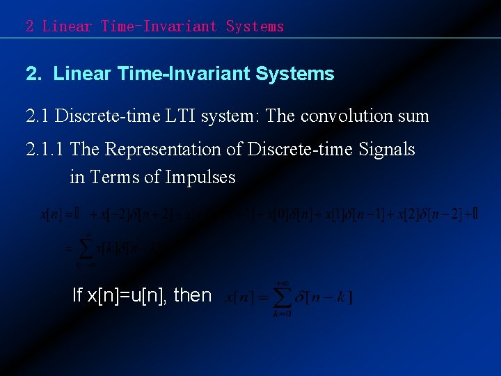
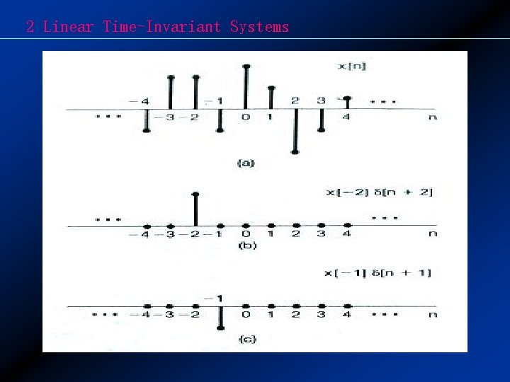
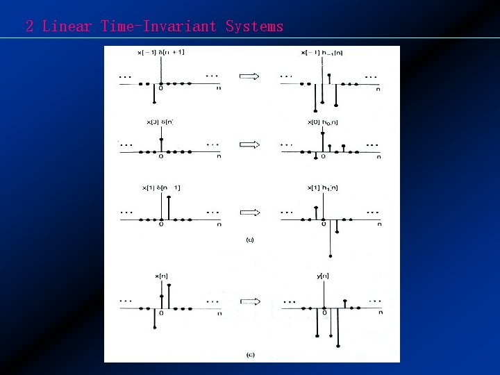
2 Linear Time-Invariant Systems 2. 1 Discrete-time LTI system: The convolution sum 2. 1. 1 The Representation of Discrete-time Signals in Terms of Impulses If x[n]=u[n], then

2 Linear Time-Invariant Systems

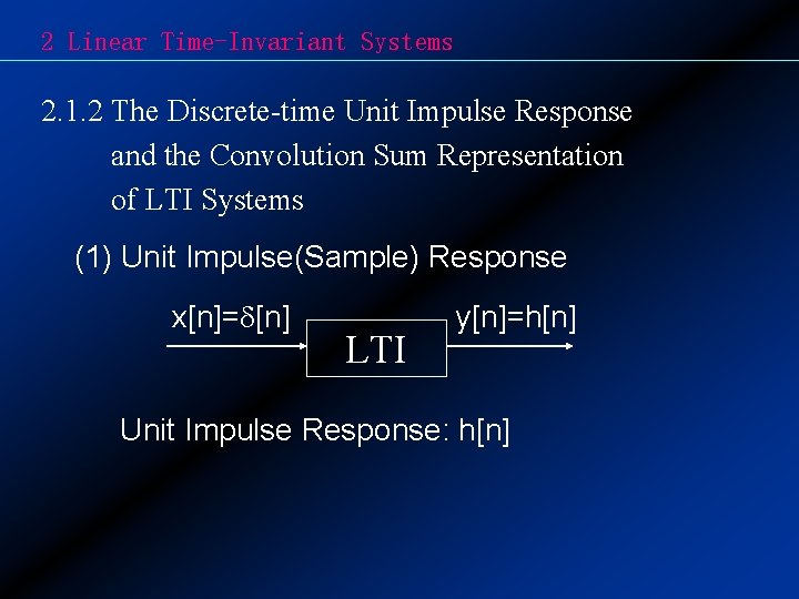
2 Linear Time-Invariant Systems 2. 1. 2 The Discrete-time Unit Impulse Response and the Convolution Sum Representation of LTI Systems (1) Unit Impulse(Sample) Response x[n]= [n] LTI y[n]=h[n] Unit Impulse Response: h[n]

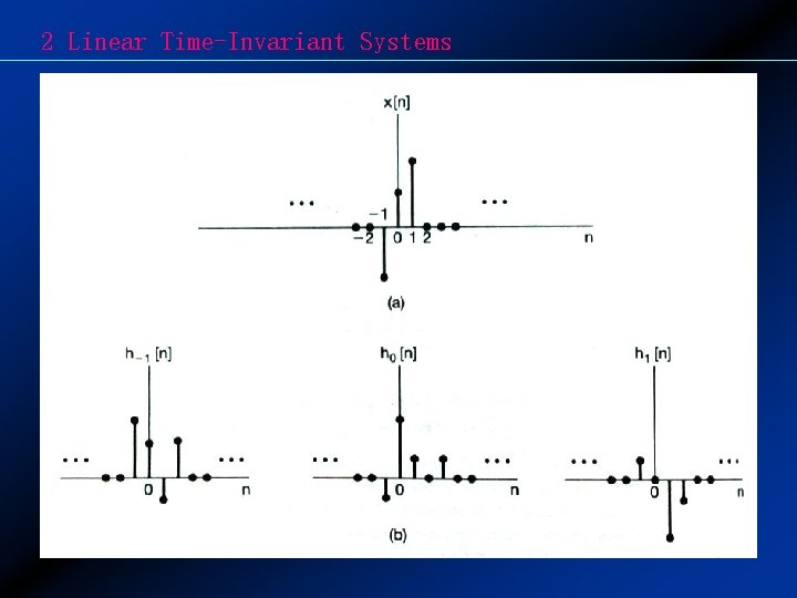
2 Linear Time-Invariant Systems (2) Convolution Sum of LTI System Question: x[n] LTI y[n]=? Solution: [n] h[n] [n-k] h[n-k] x[k] [n-k] x[k] h[n-k]

2 Linear Time-Invariant Systems

2 Linear Time-Invariant Systems

2 Linear Time-Invariant Systems So ( Convolution Sum ) or y[n] = x[n] * h[n] (3) Calculation of Convolution Sum Time Inversal: h[k] h[-k] Time Shift: h[-k] h[n-k] Multiplication: x[k]h[n-k] Summing: Example 2. 1 2. 2 2. 3 2. 4 2. 5

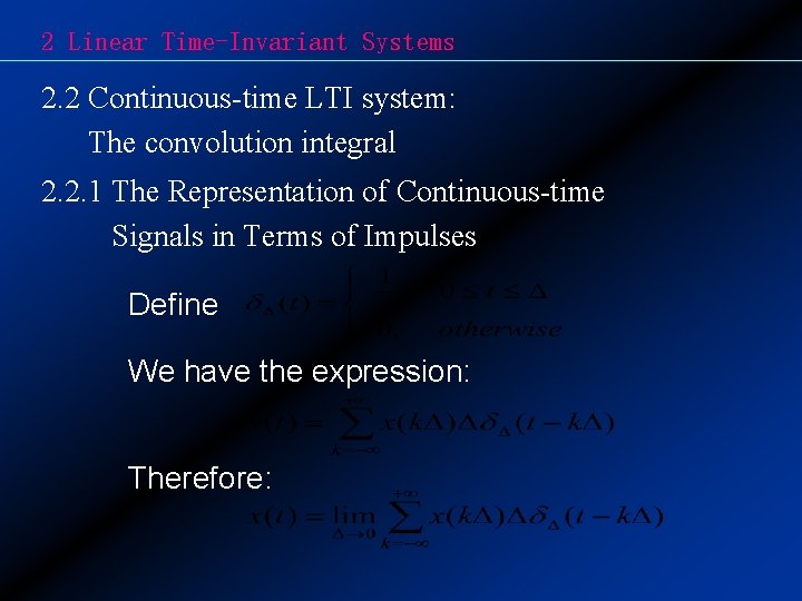
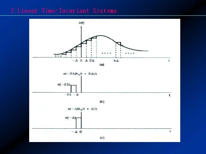
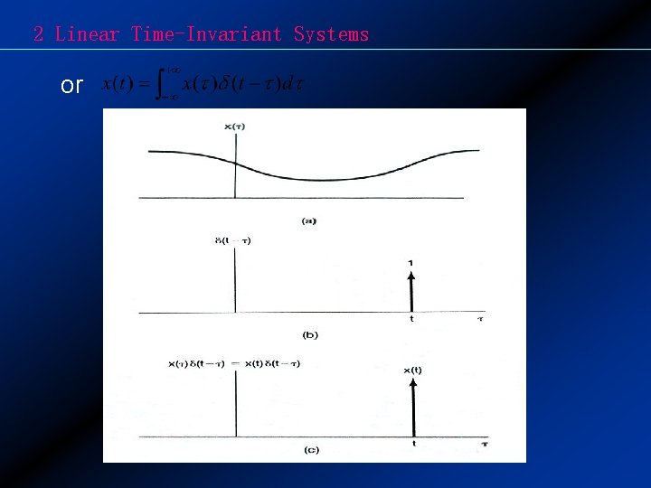
2 Linear Time-Invariant Systems 2. 2 Continuous-time LTI system: The convolution integral 2. 2. 1 The Representation of Continuous-time Signals in Terms of Impulses Define We have the expression: Therefore:

2 Linear Time-Invariant Systems

2 Linear Time-Invariant Systems or

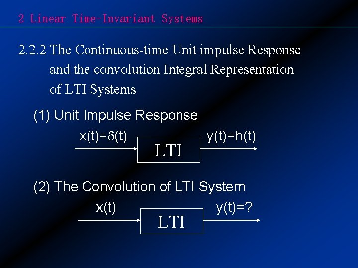
2 Linear Time-Invariant Systems 2. 2. 2 The Continuous-time Unit impulse Response and the convolution Integral Representation of LTI Systems (1) Unit Impulse Response x(t)= (t) LTI y(t)=h(t) (2) The Convolution of LTI System x(t) LTI y(t)=?

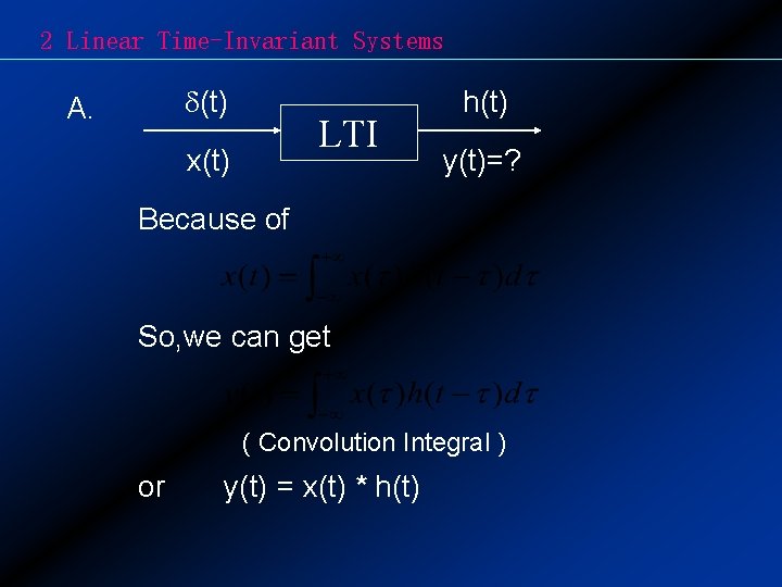
2 Linear Time-Invariant Systems (t) A. LTI x(t) h(t) y(t)=? Because of So, we can get ( Convolution Integral ) or y(t) = x(t) * h(t)

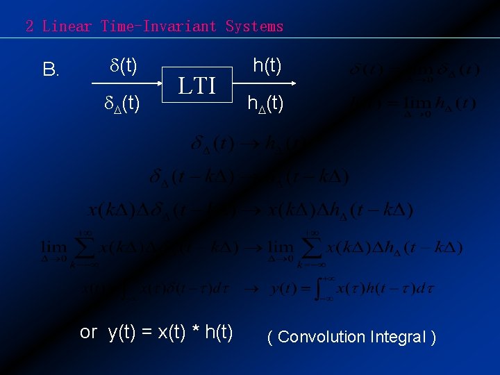
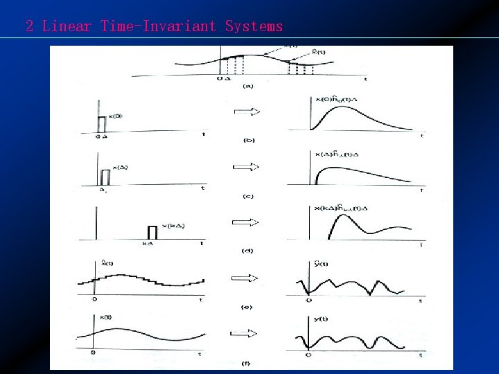
2 Linear Time-Invariant Systems B. (t) LTI or y(t) = x(t) * h(t) h (t) ( Convolution Integral )

2 Linear Time-Invariant Systems

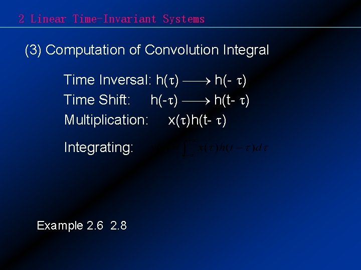
2 Linear Time-Invariant Systems (3) Computation of Convolution Integral Time Inversal: h( ) h(- ) Time Shift: h(- ) h(t- ) Multiplication: x( )h(t- ) Integrating: Example 2. 6 2. 8

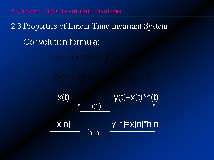
2 Linear Time-Invariant Systems 2. 3 Properties of Linear Time Invariant System Convolution formula: x(t) x[n] h(t) h[n] y(t)=x(t)*h(t) y[n]=x[n]*h[n]

2 Linear Time-Invariant Systems 2. 3. 1 The Commutative Property Discrete time: x[n]*h[n]=h[n]*x[n] Continuous time: x(t)*h(t)=h(t)*x(t) h(t) x(t) y(t)=x(t)*h(t) y(t)=h(t)*x(t)

2 Linear Time-Invariant Systems 2. 3. 2 The Distributive Property Discrete time: x[n]*{h 1[n]+h 2[n]}=x[n]*h 1[n]+x[n]*h 2[n] Continuous time: x(t)*{h 1(t)+h 2(t)}=x(t)*h 1(t)+x(t)*h 2(t) x(t) Example 2. 10 h 1(t)+h 2(t) h 1(t) h 2(t) y(t)=x(t)*{h 1(t)+h 2(t)} y(t)=x(t)*h 1(t)+x(t)*h 2(t)

2 Linear Time-Invariant Systems 2. 3. 3 The Associative Property Discrete time: x[n]*{h 1[n]*h 2[n]}={x[n]*h 1[n]}*h 2[n] Continuous time: x(t)*{h 1(t)*h 2(t)}={x(t)*h 1(t)}*h 2(t) x(t) h 1(t)*h 2(t) h 1(t) y(t)=x(t)*{h 1(t)*h 2(t)} h 2(t) y(t)=x(t)*h 1(t)*h 2(t)

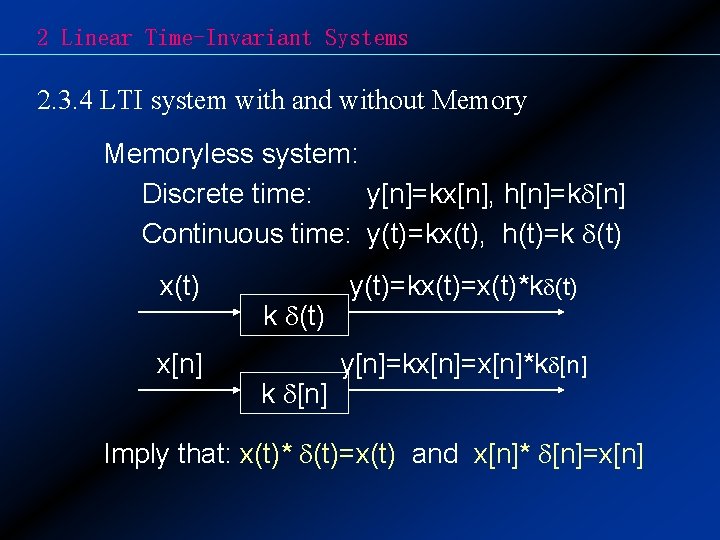
2 Linear Time-Invariant Systems 2. 3. 4 LTI system with and without Memoryless system: Discrete time: y[n]=kx[n], h[n]=k [n] Continuous time: y(t)=kx(t), h(t)=k (t) x[n] k (t) k [n] y(t)=kx(t)=x(t)*k (t) y[n]=kx[n]=x[n]*k [n] Imply that: x(t)* (t)=x(t) and x[n]* [n]=x[n]

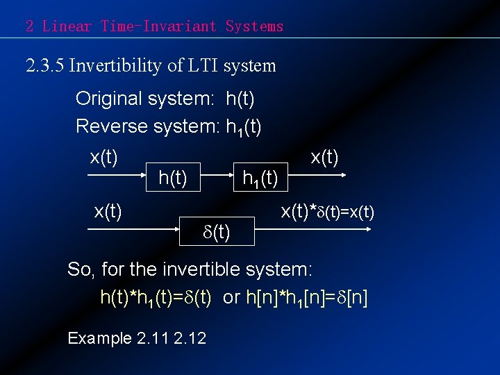
2 Linear Time-Invariant Systems 2. 3. 5 Invertibility of LTI system Original system: h(t) Reverse system: h 1(t) x(t) x(t)* (t)=x(t) So, for the invertible system: h(t)*h 1(t)= (t) or h[n]*h 1[n]= [n] Example 2. 11 2. 12

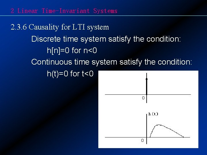
2 Linear Time-Invariant Systems 2. 3. 6 Causality for LTI system Discrete time system satisfy the condition: h[n]=0 for n<0 Continuous time system satisfy the condition: h(t)=0 for t<0

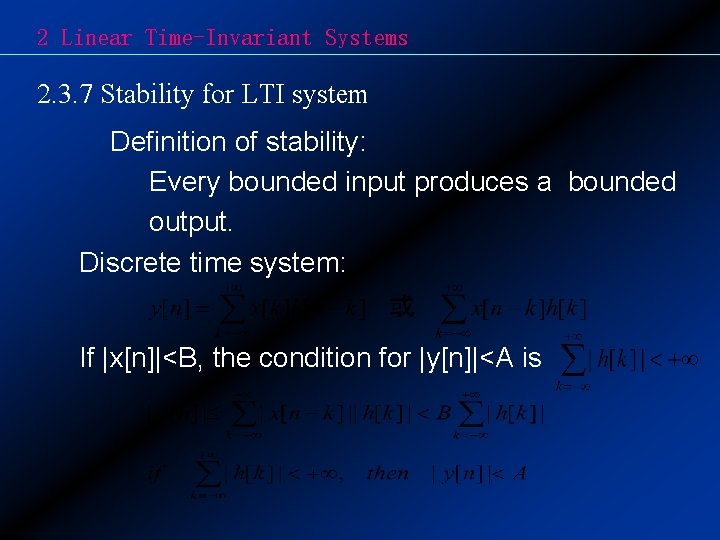
2 Linear Time-Invariant Systems 2. 3. 7 Stability for LTI system Definition of stability: Every bounded input produces a bounded output. Discrete time system: If |x[n]|<B, the condition for |y[n]|<A is

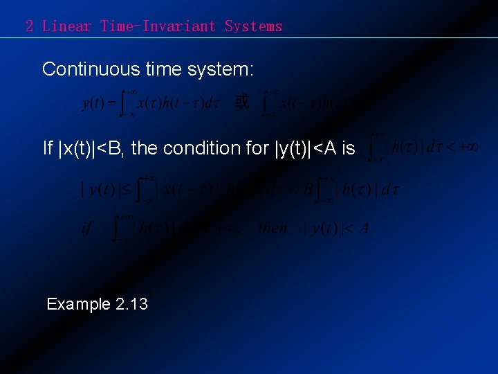
2 Linear Time-Invariant Systems Continuous time system: If |x(t)|<B, the condition for |y(t)|<A is Example 2. 13

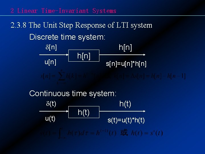
2 Linear Time-Invariant Systems 2. 3. 8 The Unit Step Response of LTI system Discrete time system: [n] u[n] h[n] s[n]=u[n]*h[n] Continuous time system: (t) u(t) h(t) s(t)=u(t)*h(t)

2 Linear Time-Invariant Systems 2. 4 Causal LTI Systems Described by Differential and Difference Equation Discrete time system: Differential Equation Continuous time system: Difference Equation

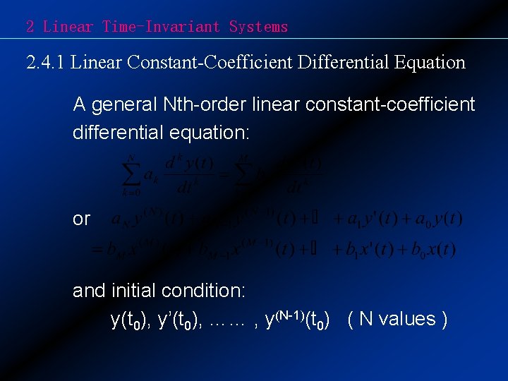
2 Linear Time-Invariant Systems 2. 4. 1 Linear Constant-Coefficient Differential Equation A general Nth-order linear constant-coefficient differential equation: or and initial condition: y(t 0), y’(t 0), …… , y(N-1)(t 0) ( N values )

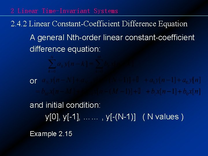
2 Linear Time-Invariant Systems 2. 4. 2 Linear Constant-Coefficient Difference Equation A general Nth-order linear constant-coefficient difference equation: or and initial condition: y[0], y[-1], …… , y[-(N-1)] ( N values ) Example 2. 15

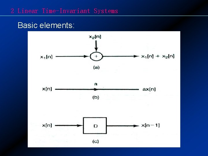
2 Linear Time-Invariant Systems 2. 4. 3 Block Diagram Representations of First-order Systems Described by Differential and Difference Equation (1) Dicrete time system Basic elements: A. An adder B. Multiplication by a coefficient C. An unit delay

2 Linear Time-Invariant Systems Basic elements:

2 Linear Time-Invariant Systems Example: y[n]+ay[n-1]=bx[n]

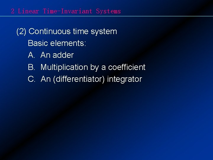
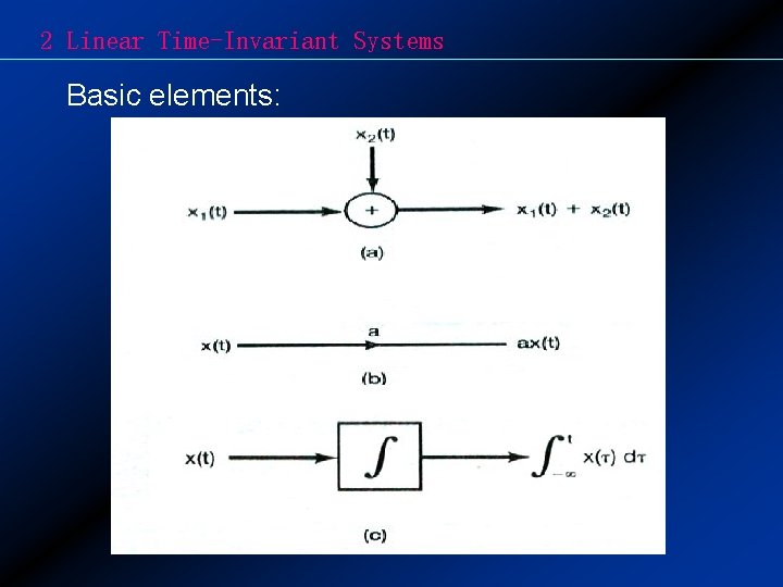
2 Linear Time-Invariant Systems (2) Continuous time system Basic elements: A. An adder B. Multiplication by a coefficient C. An (differentiator) integrator

2 Linear Time-Invariant Systems Basic elements:

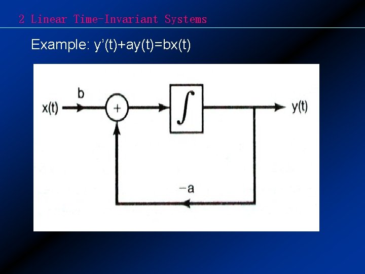
2 Linear Time-Invariant Systems Example: y’(t)+ay(t)=bx(t)

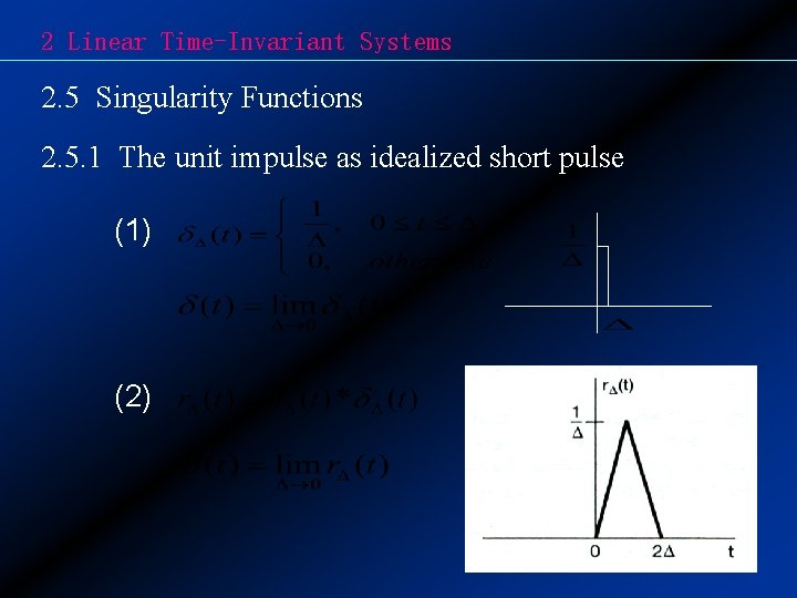
2 Linear Time-Invariant Systems 2. 5 Singularity Functions 2. 5. 1 The unit impulse as idealized short pulse (1) (2)

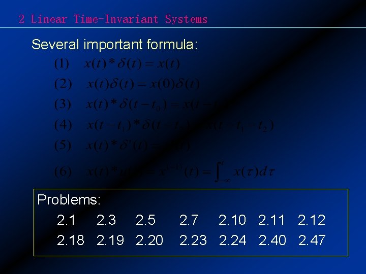
2 Linear Time-Invariant Systems Several important formula: Problems: 2. 1 2. 3 2. 5 2. 18 2. 19 2. 20 2. 7 2. 10 2. 11 2. 12 2. 23 2. 24 2. 40 2. 47