CHAPTER 2 LINEAR TIMEINVARIANT SYSTEMS 2 0 INTRODUCTION

CHAPTER 2 LINEAR TIMEINVARIANT SYSTEMS 2. 0 INTRODUCTION • LTI systems possesses the superposition(叠加) property. • Represent signals as linear combinations of delayed impulses. • Convolution sum(卷积和) or convolution integral( 卷积积分). • linear constant-coefficient difference or differential equations (线性常系数差分或微分方 程).

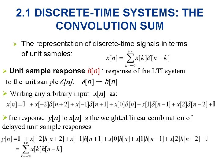
2. 1 DISCRETE-TIME SYSTEMS: THE CONVOLUTION SUM Ø The representation of discrete-time signals in terms of unit samples: Ø Unit sample response h[n] : response of the LTI system to the unit sample δ[n] → h[n] Ø Writing any arbitrary input x[n] as: Øthe response y[n] to x[n] is the weighted linear combination of delayed unit sample responses:

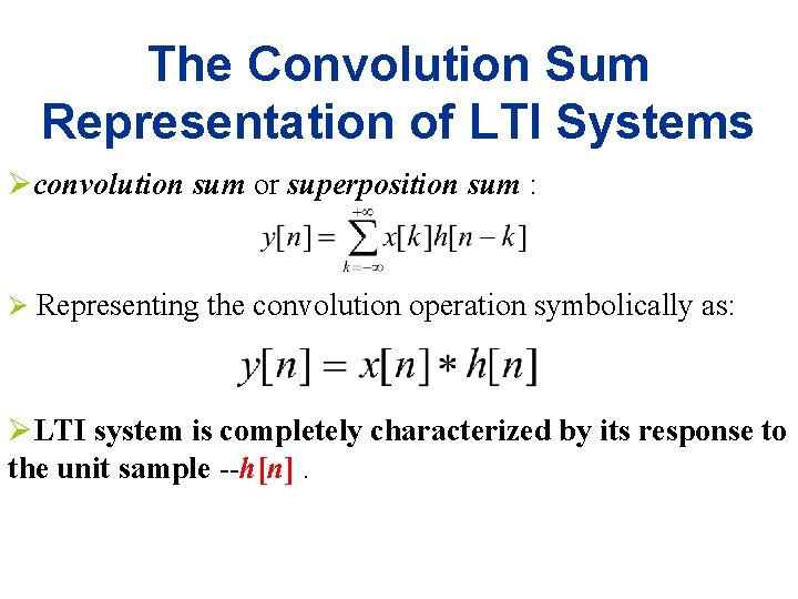
The Convolution Sum Representation of LTI Systems Øconvolution sum or superposition sum : Ø Representing the convolution operation symbolically as: ØLTI system is completely characterized by its response to the unit sample --h[n].

Example 2. 1 Consider a LTI system with unit sample response h[n] and input x[n], as illustrated in Figure (a). Calculate the convolution sum of these two sequences graphically. x[n] 0 12 h[n] n (a) -2 0 2 x[k] n h[-k] h[2] 012 k (b) h[-2] -2 0 2 k

x[k] k 012 h[n-k] If n<-2, n-2 k n+2 h[-2 -k] If n= -2, h[-2] h[2] k -4 -1 0

x[k] k 012 h[-1 -k] If n= -1, -3 k 0 1 If n=0, h[-k] -2 0 2 k

x[k] k 012 h[1 -k] If n=1, -1 0 If n=2, 3 k h[2 k] 0 2 4 k

x[k] k 012 h[3 -k] If n=3, 1 3 k 5 h[4 -k] If n=4, 0 2 3 4 5 6 k

h[n-k] If n>4, 0 n-2 n n+2 k y[n] 2. 5 2 1. 5 0. 5 -2 -1 0 1 2 3 4 Graph of y[n] in Example 2. 1 k

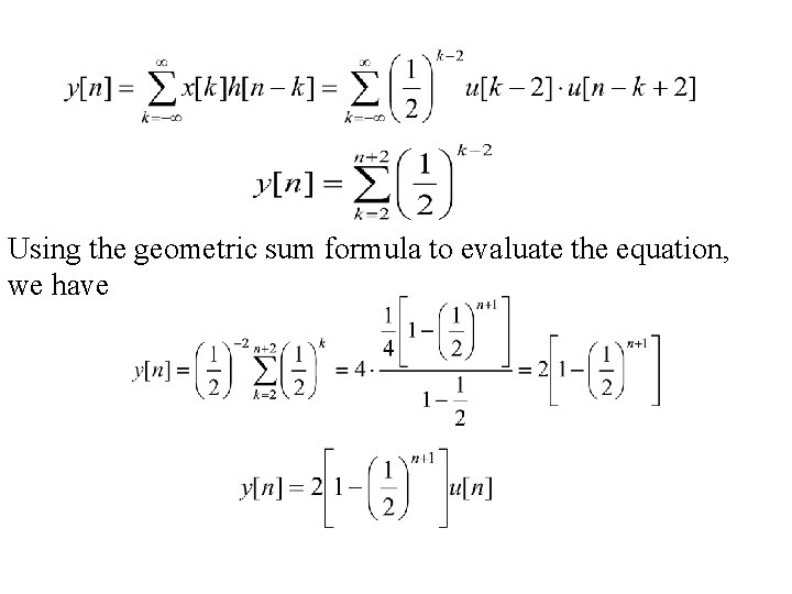
Example 2. 2 Consider an input x[n] and a unit sample response h[n] given by Determine and plot the output

Using the geometric sum formula to evaluate the equation, we have

y[n] 2 1 … … Graph of y[n] in Example 2. 2 n

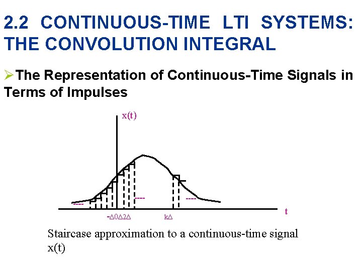
2. 2 CONTINUOUS-TIME LTI SYSTEMS: THE CONVOLUTION INTEGRAL ØThe Representation of Continuous-Time Signals in Terms of Impulses x(t) ┉ ┉ -Δ 0Δ 2Δ ┉ kΔ t Staircase approximation to a continuous-time signal x(t)

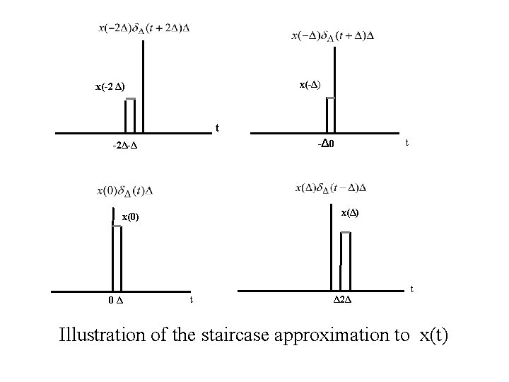
x(-Δ) x(-2 Δ) t x(Δ) x(0) 0Δ t -Δ 0 -2Δ-Δ t Δ 2Δ t Illustration of the staircase approximation to x(t)

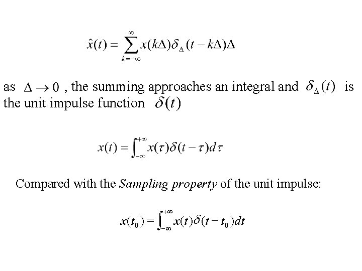
as , the summing approaches an integral and the unit impulse function Compared with the Sampling property of the unit impulse: +¥ x(t 0 ) = ò-¥ x(t )d (t - t 0 )dt is

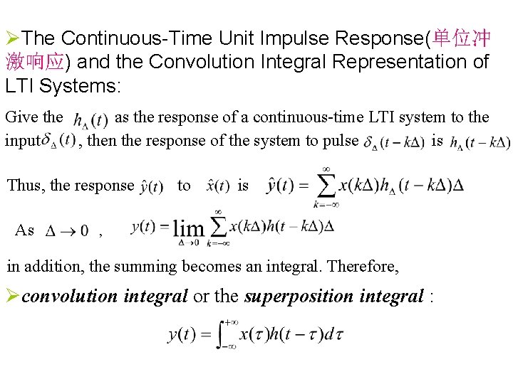
ØThe Continuous-Time Unit Impulse Response(单位冲 激响应) and the Convolution Integral Representation of LTI Systems: Give the as the response of a continuous-time LTI system to the input , then the response of the system to pulse is Thus, the response As to is , in addition, the summing becomes an integral. Therefore, Øconvolution integral or the superposition integral :

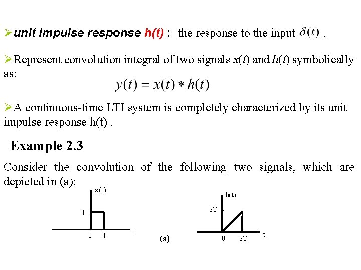
Øunit impulse response h(t) : the response to the input . ØRepresent convolution integral of two signals x(t) and h(t) symbolically as: ØA continuous-time LTI system is completely characterized by its unit impulse response h(t). Example 2. 3 Consider the convolution of the following two signals, which are depicted in (a): x(t) h(t) 2 T 1 0 T t (a) 0 2 T t

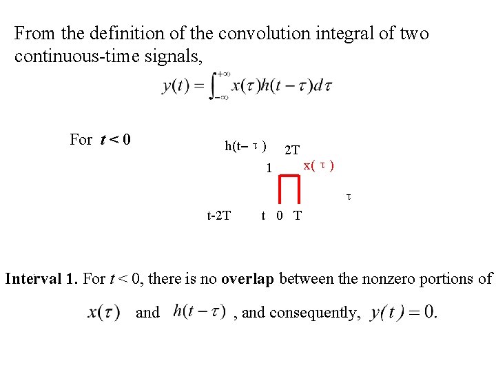
From the definition of the convolution integral of two continuous-time signals, For t < 0 h(t–τ) 2 T 1 x(τ) τ t-2 T t 0 T . Interval 1. For t < 0, there is no overlap between the nonzero portions of and , and consequently,

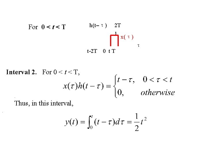
For 0 < t < T h(t–τ) t-2 T Interval 2. For 0 < t < T, . Thus, in this interval, . 2 T 1 0 t. T x(τ) τ

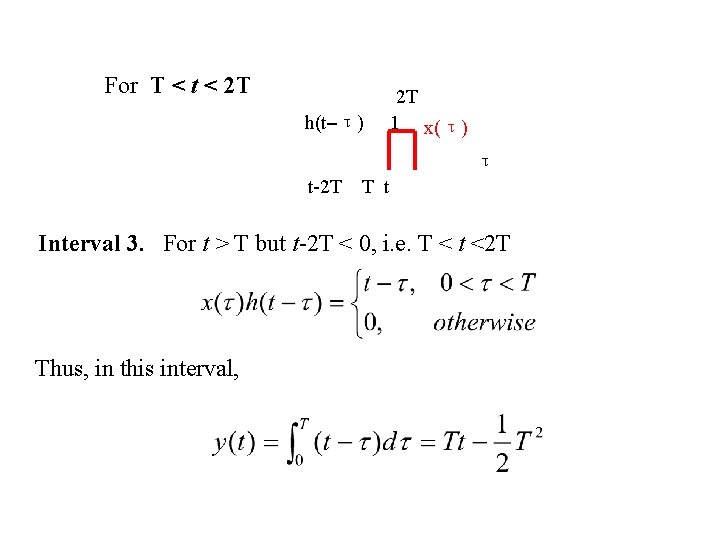
For T < t < 2 T h(t–τ) 2 T 1 x(τ) τ t-2 T T t Interval 3. For t > T but t-2 T < 0, i. e. T < t <2 T Thus, in this interval,

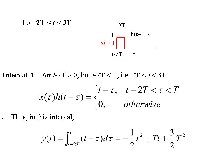
For 2 T < t < 3 T 2 T 1 x(τ) t-2 T h(t–τ) τ t Interval 4. For t-2 T > 0, but t-2 T < T, i. e. 2 T < t < 3 T . Thus, in this interval,

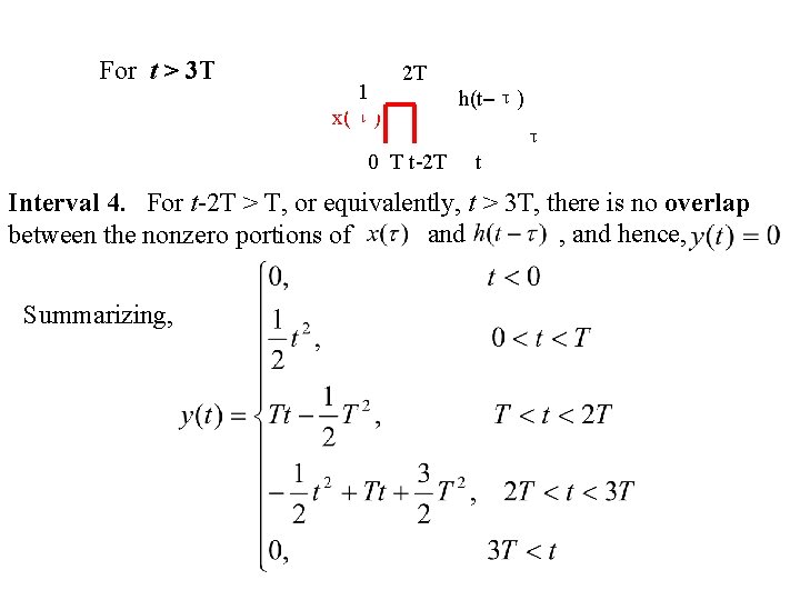
For t > 3 T 1 x(τ) 2 T 0 T t-2 T h(t–τ) τ t Interval 4. For t-2 T > T, or equivalently, t > 3 T, there is no overlap and , and hence, between the nonzero portions of Summarizing,

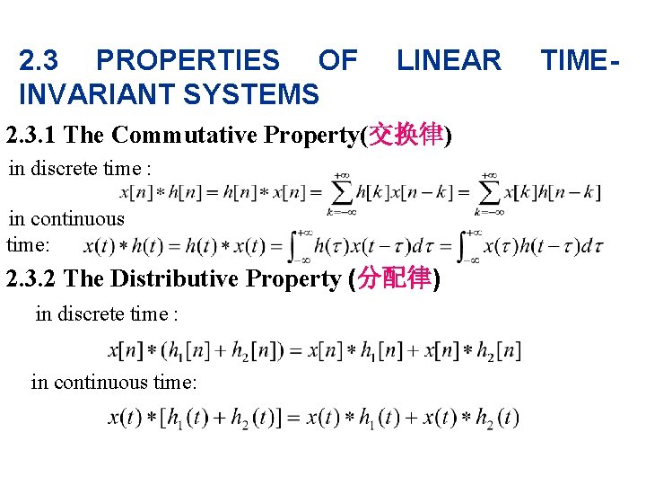
2. 3 PROPERTIES OF INVARIANT SYSTEMS LINEAR 2. 3. 1 The Commutative Property(交换律) in discrete time : in continuous time: 2. 3. 2 The Distributive Property (分配律) in discrete time : in continuous time: TIME-

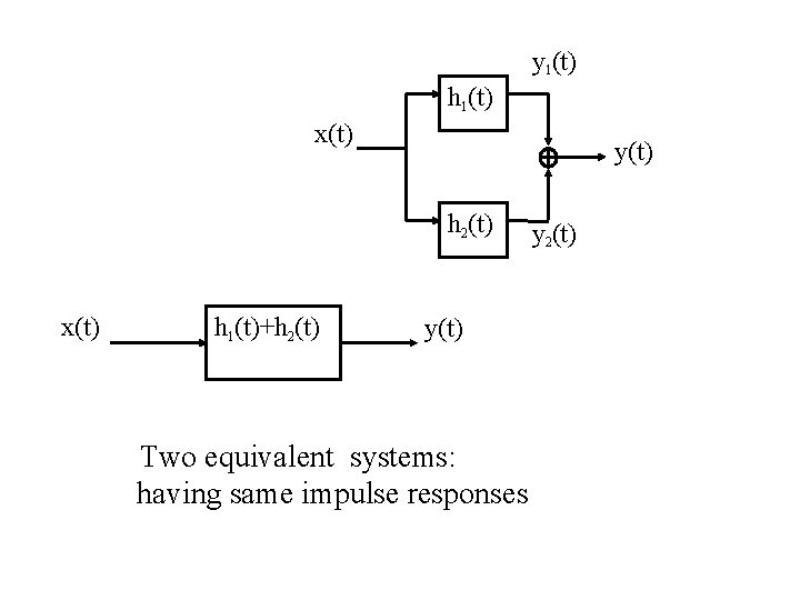
y 1(t) h 1(t) x(t) y(t) h 2(t) x(t) h 1(t)+h 2(t) y(t) Two equivalent systems: having same impulse responses y 2(t)

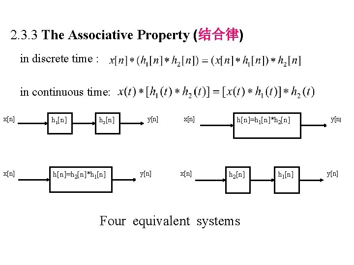
2. 3. 3 The Associative Property (结合律) in discrete time : in continuous time: x[n] h 1[n] x[n] h[n]=h 2[n]*h 1[n] h 2[n] y[n] x[n] h[n]=h 1[n]*h 2[n] Four equivalent systems h 1[n] y[n]

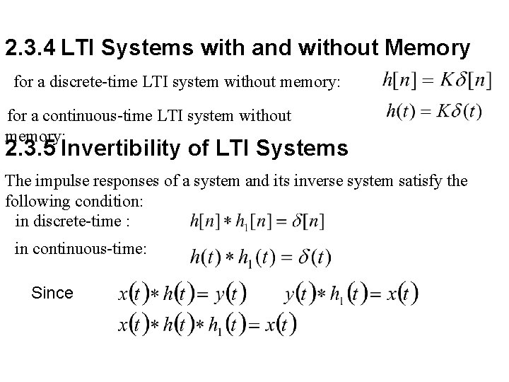
2. 3. 4 LTI Systems with and without Memory for a discrete-time LTI system without memory: for a continuous-time LTI system without memory: 2. 3. 5 Invertibility of LTI Systems The impulse responses of a system and its inverse system satisfy the following condition: in discrete-time : in continuous-time: Since

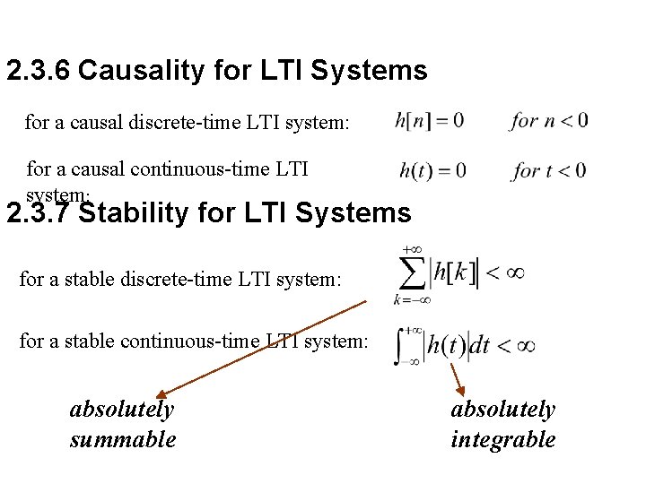
2. 3. 6 Causality for LTI Systems for a causal discrete-time LTI system: for a causal continuous-time LTI system: 2. 3. 7 Stability for LTI Systems for a stable discrete-time LTI system: for a stable continuous-time LTI system: absolutely summable absolutely integrable

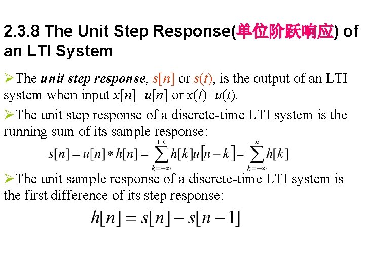
2. 3. 8 The Unit Step Response(单位阶跃响应) of an LTI System ØThe unit step response, s[n] or s(t), is the output of an LTI system when input x[n]=u[n] or x(t)=u(t). ØThe unit step response of a discrete-time LTI system is the running sum of its sample response: ØThe unit sample response of a discrete-time LTI system is the first difference of its step response:

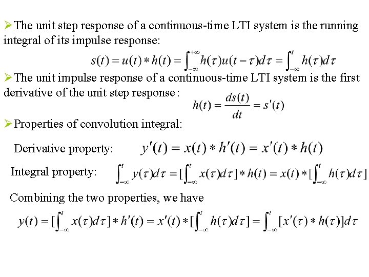
ØThe unit step response of a continuous-time LTI system is the running integral of its impulse response: ØThe unit impulse response of a continuous-time LTI system is the first derivative of the unit step response : ØProperties of convolution integral: Derivative property: Integral property: Combining the two properties, we have

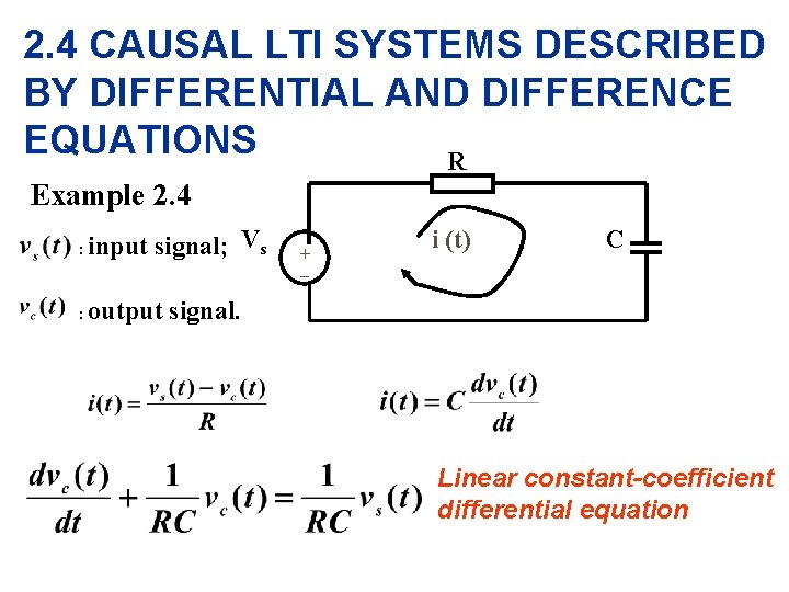
2. 4 CAUSAL LTI SYSTEMS DESCRIBED BY DIFFERENTIAL AND DIFFERENCE EQUATIONS R Example 2. 4 : input signal; Vs : output signal. + – i (t) C Linear constant-coefficient differential equation

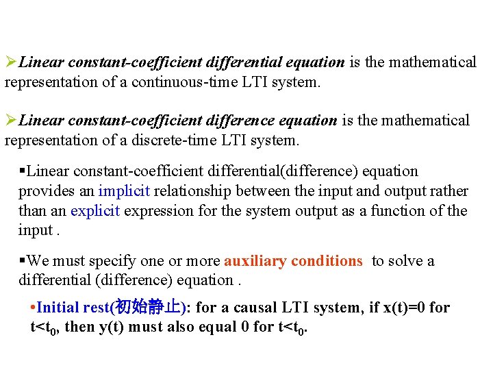
ØLinear constant-coefficient differential equation is the mathematical representation of a continuous-time LTI system. ØLinear constant-coefficient difference equation is the mathematical representation of a discrete-time LTI system. §Linear constant-coefficient differential(difference) equation provides an implicit relationship between the input and output rather than an explicit expression for the system output as a function of the input. §We must specify one or more auxiliary conditions to solve a differential (difference) equation. • Initial rest(初始静止): for a causal LTI system, if x(t)=0 for t<t 0, then y(t) must also equal 0 for t<t 0.

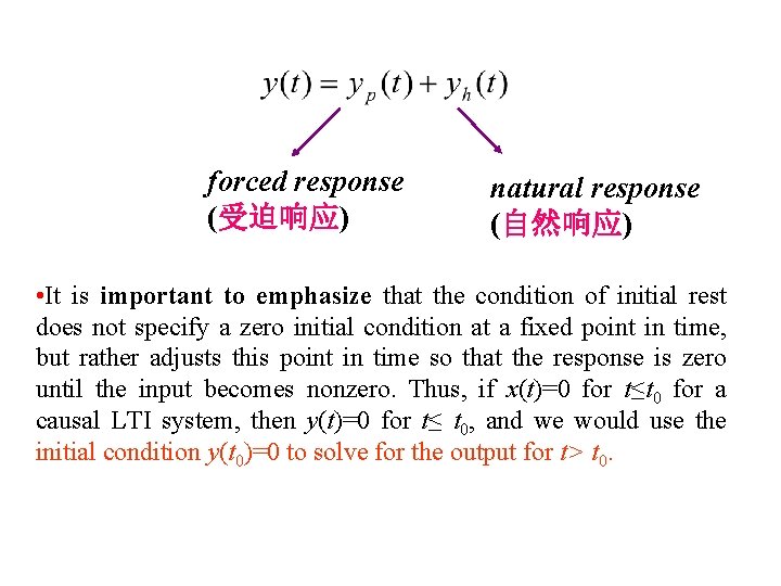
forced response (受迫响应) natural response (自然响应) • It is important to emphasize that the condition of initial rest does not specify a zero initial condition at a fixed point in time, but rather adjusts this point in time so that the response is zero until the input becomes nonzero. Thus, if x(t)=0 for t≤t 0 for a causal LTI system, then y(t)=0 for t≤ t 0, and we would use the initial condition y(t 0)=0 to solve for the output for t> t 0.

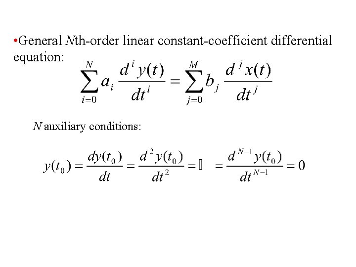
• General Nth-order linear constant-coefficient differential equation: N auxiliary conditions:

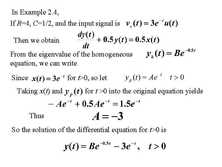
In Example 2. 4, If R=4, C=1/2, and the input signal is Then we obtain From the eigenvalue of the homogeneous equation, we can write Since for t>0, so let Taking x(t) and for t >0 into the original equation yields Thus So the solution of the differential equation for t>0 is

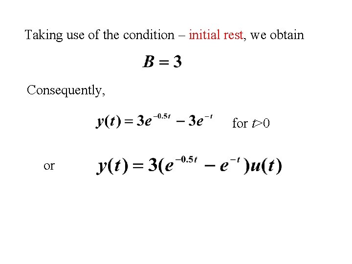
Taking use of the condition – initial rest, we obtain Consequently, for t>0 or

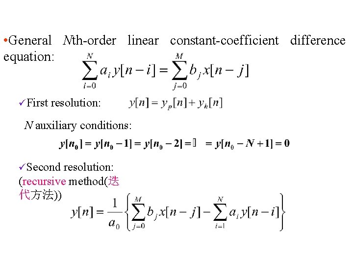
• General Nth-order linear constant-coefficient difference equation: üFirst resolution: N auxiliary conditions: üSecond resolution: (recursive method(迭 代方法))

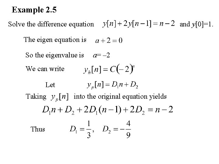
Example 2. 5 Solve the difference equation The eigen equation is So the eigenvalue is a= – 2 We can write Let Taking Thus into the original equation yields and y[0]=1.

The solution for the given equation is From the initial condition of y[0]=1, we have Consequently,

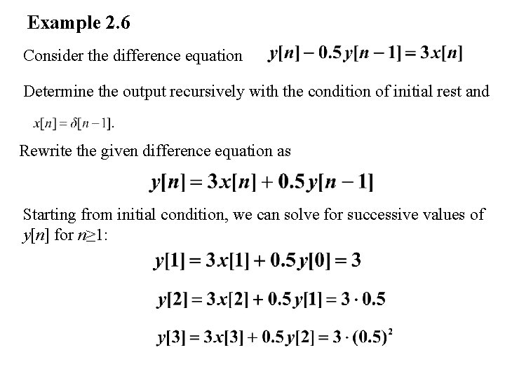
Example 2. 6 Consider the difference equation Determine the output recursively with the condition of initial rest and Rewrite the given difference equation as . Starting from initial condition, we can solve for successive values of y[n] for n≥ 1:

Considering y[n] =0 for n≤ 0, the solution is

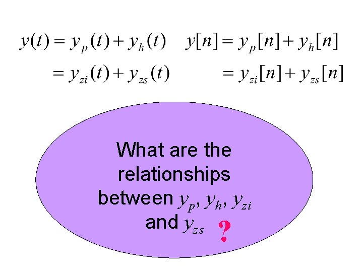
What are the relationships between yp, yh, yzi and yzs ?

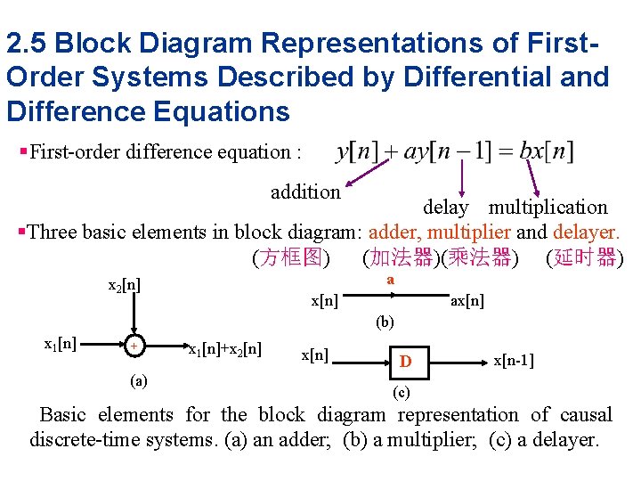
2. 5 Block Diagram Representations of First. Order Systems Described by Differential and Difference Equations §First-order difference equation : addition delay multiplication §Three basic elements in block diagram: adder, multiplier and delayer. (方框图) (加法器)(乘法器) (延时器) a x 2[n] x[n] ax[n] (b) x 1[n] + (a) x 1[n]+x 2[n] x[n] D x[n-1] (c) Basic elements for the block diagram representation of causal discrete-time systems. (a) an adder; (b) a multiplier; (c) a delayer.

x[n] b y[n] + D -a y[n-1] Block diagram representation for the causal discrete-time system described by the first-order difference equation (y[n]+ay[n-1]=bx[n]). §First-order differential equation : differentiation

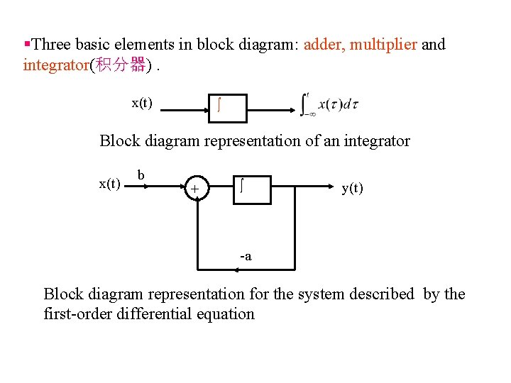
§Three basic elements in block diagram: adder, multiplier and integrator(积分器). x(t) ∫ Block diagram representation of an integrator x(t) b + ∫ y(t) -a Block diagram representation for the system described by the first-order differential equation

2. 6 SUMMARY ØA representation of an arbitrary discrete-time signal as weighted sums of shifted unit samples; ØConvolution sum representation for the response of a discrete-time LTI systems; ØA representation of an arbitrary continuous-time signal a weighted integrals of shifted unit impulses; ØConvolution integral representation for continuous-time LTI systems; ØRelating LTI system properties, including causality, stability, to corresponding properties of the unit impulse (sample) response; ØSome of the properties of systems described by linear constant-coefficient differential (difference) equations; ØUnderstanding of the condition of initial rest.