Appendix 02 Linear Systems Timeinvariant systems ft Linear

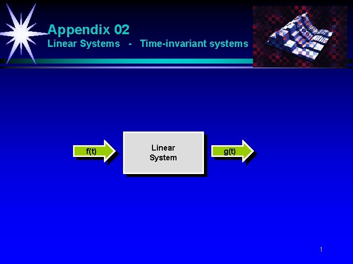
Appendix 02 Linear Systems - Time-invariant systems f(t) Linear System g(t) 1

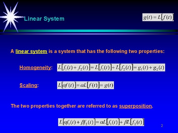
Linear System A linear system is a system that has the following two properties: Homogeneity: Scaling: The two properties together are referred to as superposition. 2

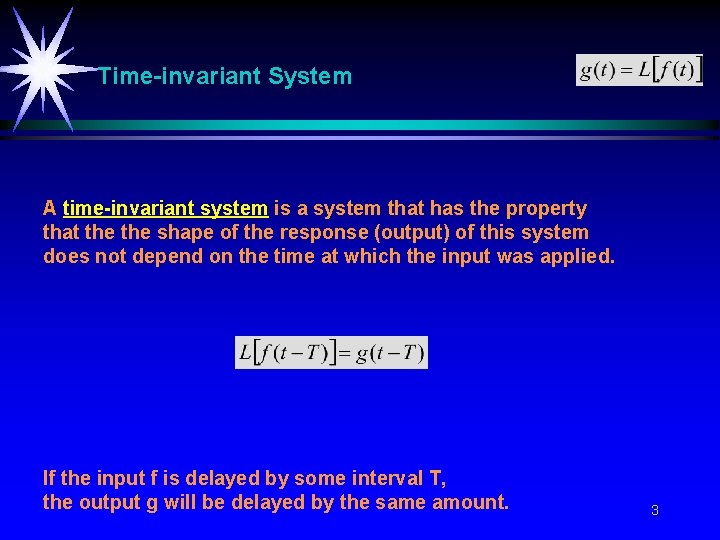
Time-invariant System A time-invariant system is a system that has the property that the shape of the response (output) of this system does not depend on the time at which the input was applied. If the input f is delayed by some interval T, the output g will be delayed by the same amount. 3

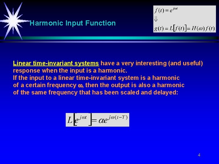
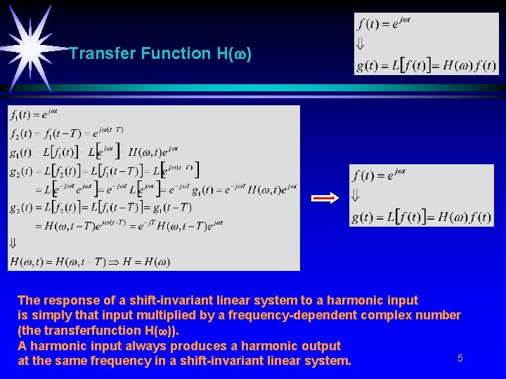
Harmonic Input Function Linear time-invariant systems have a very interesting (and useful) response when the input is a harmonic. If the input to a linear time-invariant system is a harmonic of a certain frequency , then the output is also a harmonic of the same frequency that has been scaled and delayed: 4

Transfer Function H( ) The response of a shift-invariant linear system to a harmonic input is simply that input multiplied by a frequency-dependent complex number (the transferfunction H( )). A harmonic input always produces a harmonic output 5 at the same frequency in a shift-invariant linear system.

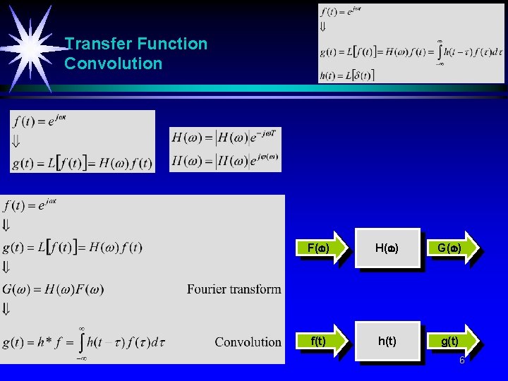
Transfer Function Convolution F( ) H( ) G( ) f(t) h(t) g(t) 6

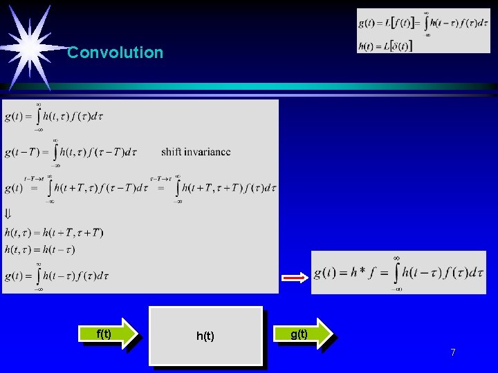
Convolution f(t) h(t) g(t) 7

Impulse Response [1/4] 8

Impulse Response [2/4] f(t) h(t) g(t) F( ) H( ) G( ) 9

Impulse Response [3/4] Convolution g(t) t 10

Impulse Response [4/4] Convolution = * 11

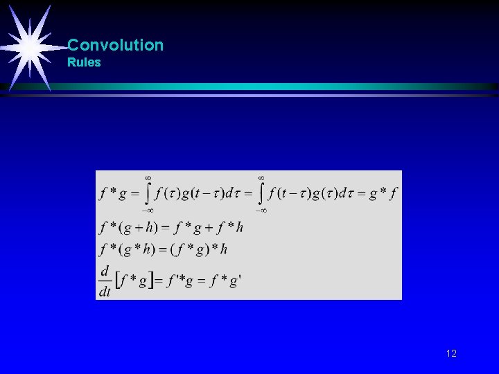
Convolution Rules 12

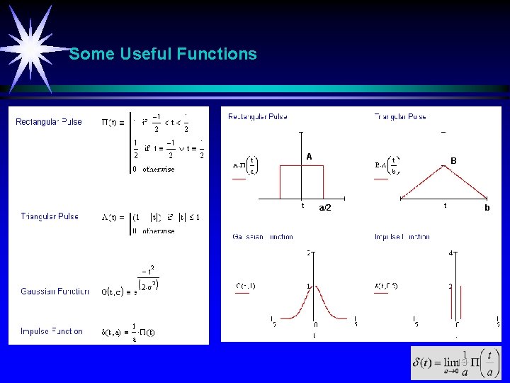
Some Useful Functions A B a/2 b 13

The Impulse Function [1/2] The impulse is the identity function under convolution 14

The Impulse Function [2/2] 15

Step Function [1/3] b b 16

Step Function [2/3] b b 17

Step Function [3/3] b 18

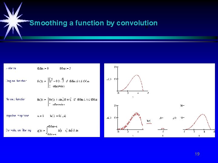
Smoothing a function by convolution b 19

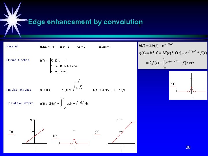
Edge enhancement by convolution b 20

Discrete 1 -Dim Convolution [1/5] Matrix 21

Discrete 1 -Dim Convolution [2/5] Example 22

Discrete 1 -Dim Convolution [3/5] Discrete operation 23

Discrete 1 -Dim Convolution [4/5] Graph - Continuous / Discrete 24

Discrete 1 -Dim Convolution [5/5] Wrapping h index array 25

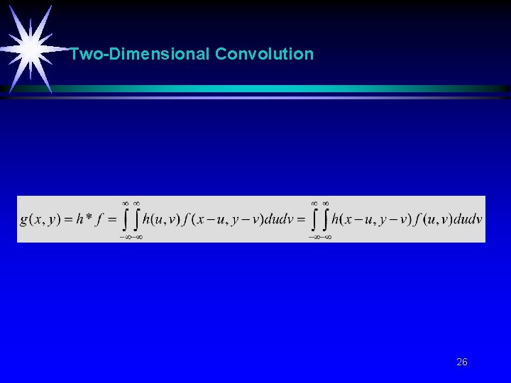
Two-Dimensional Convolution 26

Discrete Two-Dimensional Convolution [1/3] 27

Discrete Two-Dimensional Convolution [2/3] 28

Discrete Two-Dimensional Convolution [3/3] Kernel matrix Input image Array of products Output image Summer x. C Scaling factor Output pixel 29

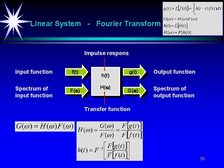
Linear System - Fourier Transform Impulse respons Input function f(t) Spectrum of input function F( ) h(t) H( ) g(t) Output function G( ) Spectrum of output function Transfer function 30

End 31