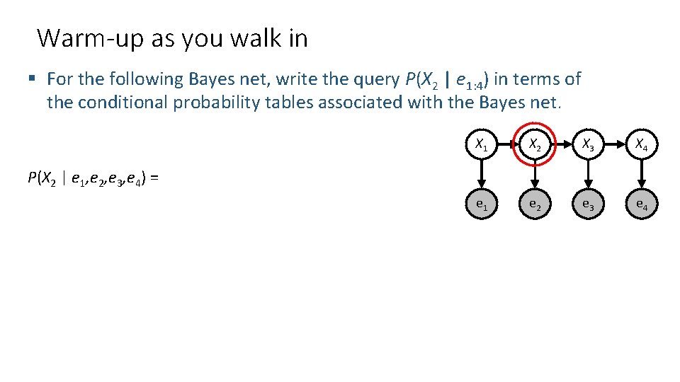
Warmup as you walk in For the following

Warm-up as you walk in § For the following Bayes net, write the query P(X 2 | e 1: 4) in terms of the conditional probability tables associated with the Bayes net. X 1 X 2 X 3 X 4 e 1 e 2 e 3 e 4 P(X 2 | e 1, e 2, e 3, e 4) =

Announcements Assignments § HW 10 § Due Wed 11/20 § P 5 § Due Mon 11/25 § HW 11 § Out tonight § Due Tue 11/28 Wed 11/27 In-class Polls § Denominator capped after 11/14 lecture, 74 polls

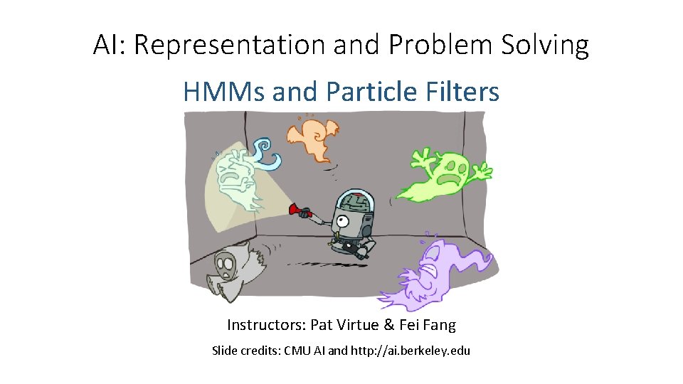
AI: Representation and Problem Solving HMMs and Particle Filters Instructors: Pat Virtue & Fei Fang Slide credits: CMU AI and http: //ai. berkeley. edu

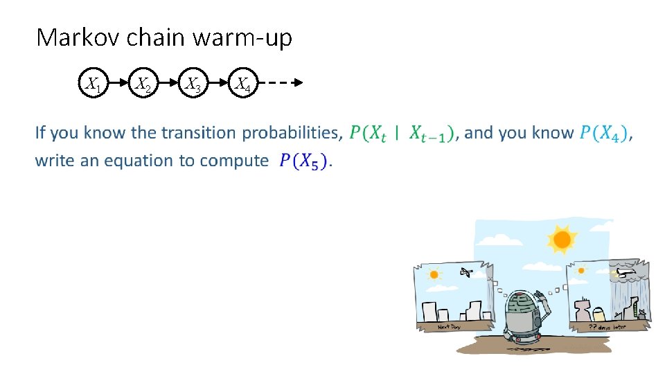
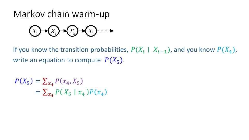
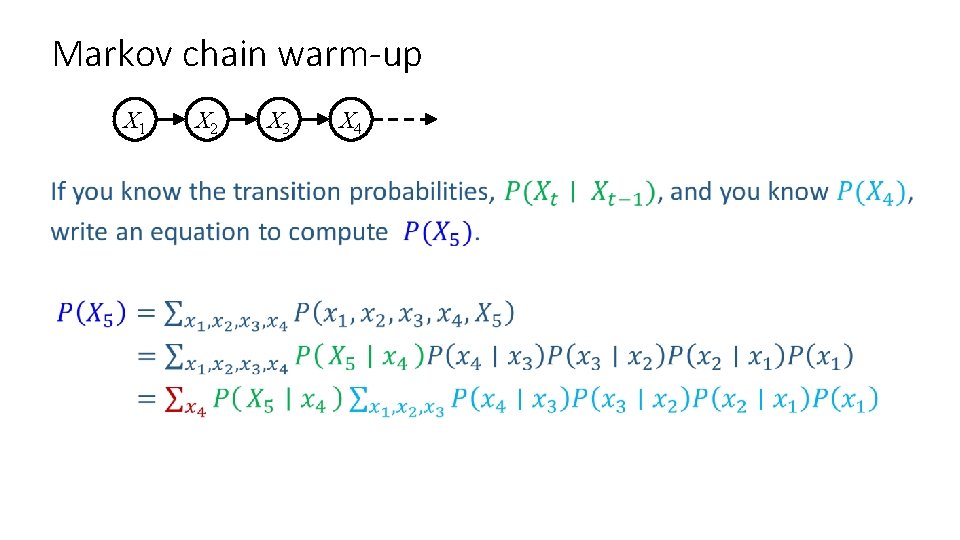
Markov chain warm-up X 1 X 2 X 3 X 4

Markov chain warm-up X 1 X 2 X 3 X 4

Markov chain warm-up X 1 X 2 X 3 X 4

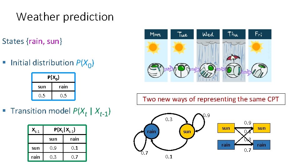
Weather prediction States {rain, sun} § Initial distribution P(X 0) sun rain 0. 5 Two new ways of representing the same CPT § Transition model P(Xt | Xt-1) Xt-1 P(Xt|Xt-1) sun rain sun 0. 9 0. 1 rain 0. 3 0. 7 0. 9 0. 3 rain sun rain 0. 7 0. 1 0. 9 0. 1 0. 3 0. 7 sun rain

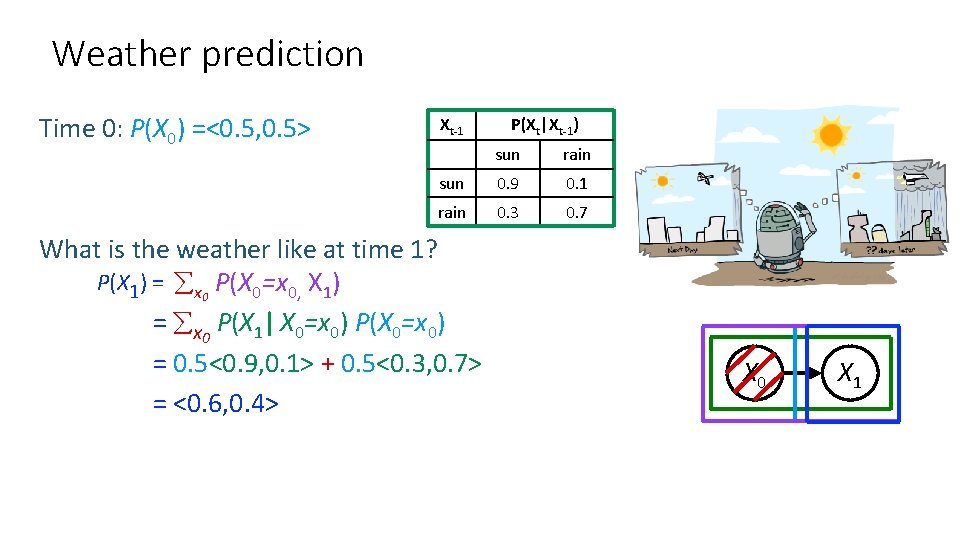
Weather prediction Time 0: P(X 0) =<0. 5, 0. 5> Xt-1 P(Xt|Xt-1) sun rain sun 0. 9 0. 1 rain 0. 3 0. 7 What is the weather like at time 1? P(X 1) = x 0 P(X 0=x 0, X 1) = x 0 P(X 1| X 0=x 0) P(X 0=x 0) = 0. 5<0. 9, 0. 1> + 0. 5<0. 3, 0. 7> = <0. 6, 0. 4> X 0 X 1

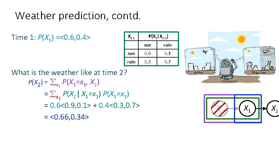
Weather prediction, contd. Time 1: P(X 1) =<0. 6, 0. 4> Xt-1 P(Xt|Xt-1) sun rain sun 0. 9 0. 1 rain 0. 3 0. 7 What is the weather like at time 2? P(X 2) = x 1 P(X 1=x 1, X 2) = x 1 P(X 2| X 1=x 1) P(X 1=x 1) = 0. 6<0. 9, 0. 1> + 0. 4<0. 3, 0. 7> = <0. 66, 0. 34> X 0 X 1 X 2

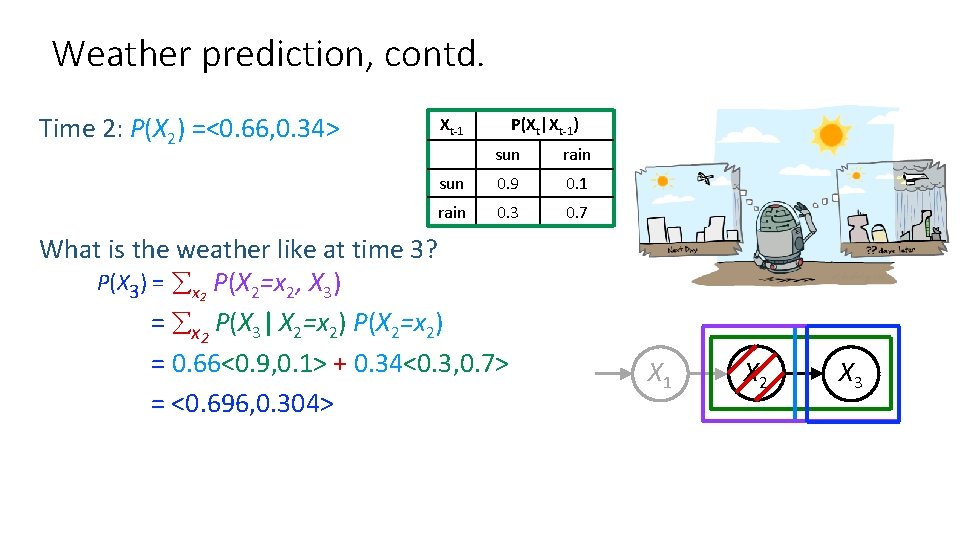
Weather prediction, contd. Time 2: P(X 2) =<0. 66, 0. 34> Xt-1 P(Xt|Xt-1) sun rain sun 0. 9 0. 1 rain 0. 3 0. 7 What is the weather like at time 3? P(X 3) = x 2 P(X 2=x 2, X 3) = x 2 P(X 3| X 2=x 2) P(X 2=x 2) = 0. 66<0. 9, 0. 1> + 0. 34<0. 3, 0. 7> = <0. 696, 0. 304> X 1 X 2 X 3

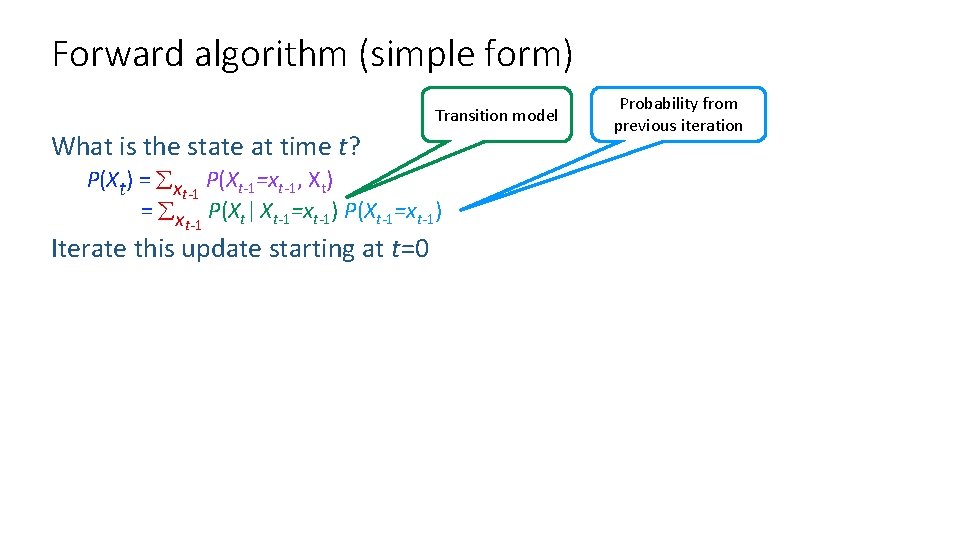
Forward algorithm (simple form) Transition model What is the state at time t? P(Xt) = x P(Xt-1=xt-1, Xt) t-1 = x P(Xt| Xt-1=xt-1) P(Xt-1=xt-1) t-1 Iterate this update starting at t=0 Probability from previous iteration

Hidden Markov Models

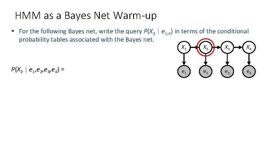
HMM as a Bayes Net Warm-up § For the following Bayes net, write the query P(X 2 | e 1: 4) in terms of the conditional probability tables associated with the Bayes net. P(X 2 | e 1, e 2, e 3, e 4) = X 1 X 2 X 3 X 4 e 1 e 2 e 3 e 4

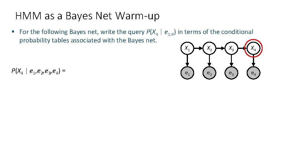
HMM as a Bayes Net Warm-up § For the following Bayes net, write the query P(X 4 | e 1: 4) in terms of the conditional probability tables associated with the Bayes net. P(X 4 | e 1, e 2, e 3, e 4) = X 1 X 2 X 3 X 4 e 1 e 2 e 3 e 4

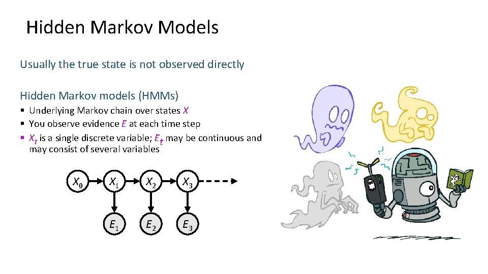
Hidden Markov Models Usually the true state is not observed directly Hidden Markov models (HMMs) § Underlying Markov chain over states X § You observe evidence E at each time step § Xt is a single discrete variable; Et may be continuous and may consist of several variables X 0 X 1 X 2 X 3 X 5 E 1 E 2 E 3 E 5

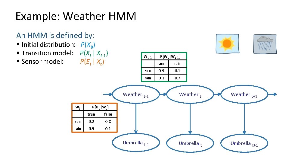
Example: Weather HMM An HMM is defined by: § Initial distribution: P(X 0) § Transition model: P(Xt | Xt-1) § Sensor model: P(Et | Xt) Wt Wt-1 P(Wt|Wt-1 ) sun rain sun 0. 9 0. 1 rain 0. 3 0. 7 Weather t-1 Weather t+1 Umbrella t-1 Umbrella t+1 P(Ut|Wt) true false sun 0. 2 0. 8 rain 0. 9 0. 1

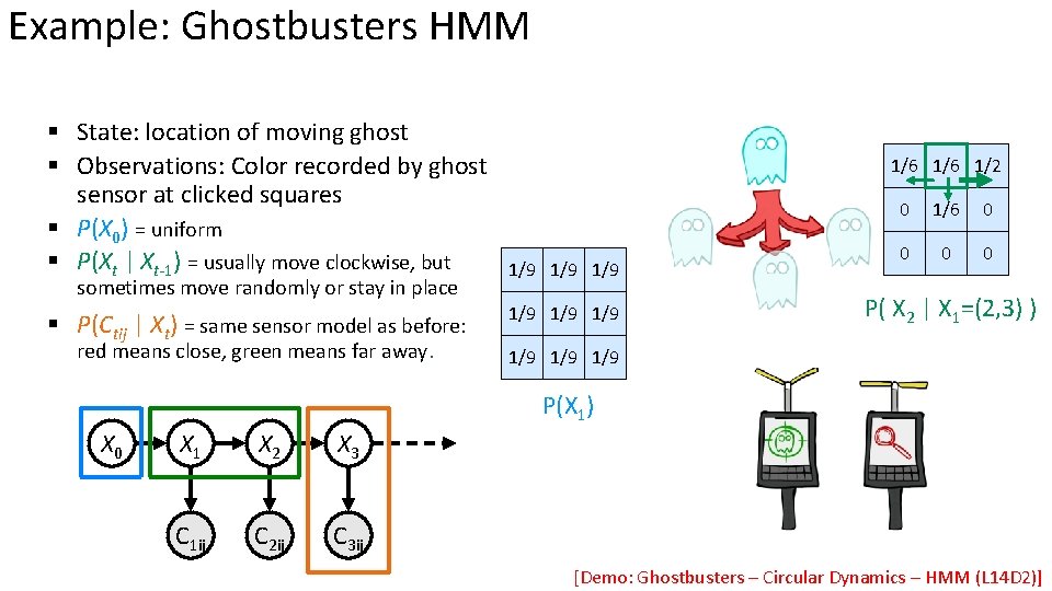
Example: Ghostbusters HMM § State: location of moving ghost § Observations: Color recorded by ghost sensor at clicked squares § P(X 0) = uniform § P(Xt | Xt-1) = usually move clockwise, but sometimes move randomly or stay in place 1/6 1/2 1/9 1/9 1/9 § P(Ctij | Xt) = same sensor model as before: red means close, green means far away. 0 1/6 0 0 P( X 2 | X 1=(2, 3) ) 1/9 1/9 P(X 1) X 0 X 1 X 2 X 3 X 5 C 1 ij C 2 ij C 3 ij [Demo: Ghostbusters – Circular Dynamics – HMM (L 14 D 2)]

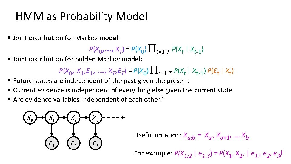
HMM as Probability Model § Joint distribution for Markov model: P(X 0, …, XT) = P(X 0) t=1: T P(Xt | Xt-1) § Joint distribution for hidden Markov model: P(X 0, X 1, E 1, …, XT, ET) = P(X 0) t=1: T P(Xt | Xt-1) P(Et | Xt) § Future states are independent of the past given the present § Current evidence is independent of everything else given the current state § Are evidence variables independent of each other? X 0 X 1 E 1 X 2 E 2 X 3 E 3 X 5 Useful notation: Xa: b = Xa , Xa+1, …, Xb E 5 For example: P(X 1: 2 | e 1: 3) = P(X 1, X 2, | e 1 , e 2, e 3)

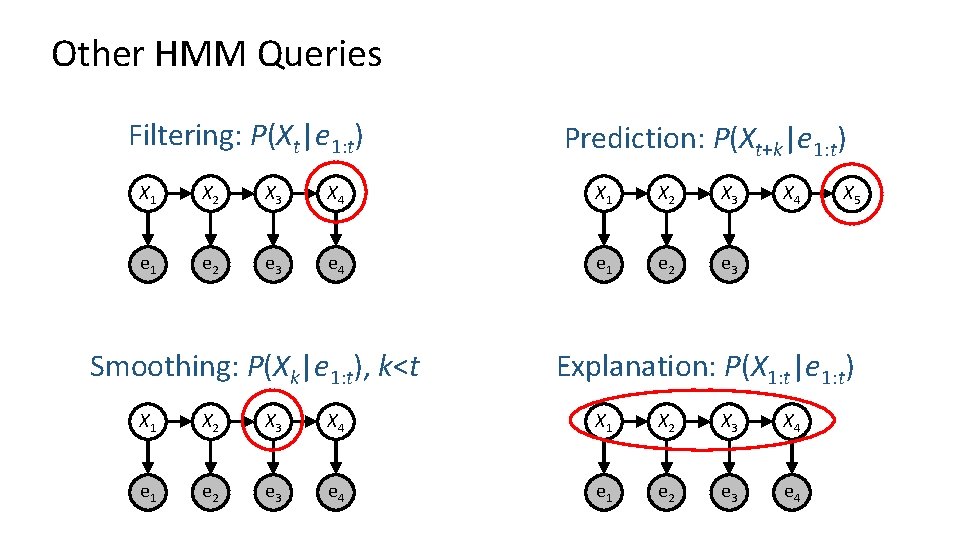
Other HMM Queries Filtering: P(Xt|e 1: t) Prediction: P(Xt+k|e 1: t) X 1 X 2 X 3 X 4 X 1 X 2 X 3 e 1 e 2 e 3 e 4 e 1 e 2 e 3 Smoothing: P(Xk|e 1: t), k<t X 4 X 5 Explanation: P(X 1: t|e 1: t) X 1 X 2 X 3 X 4 e 1 e 2 e 3 e 4

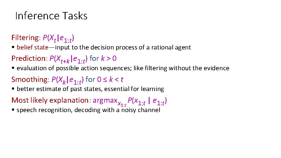
Inference Tasks Filtering: P(Xt|e 1: t) § belief state—input to the decision process of a rational agent Prediction: P(Xt+k|e 1: t) for k > 0 § evaluation of possible action sequences; like filtering without the evidence Smoothing: P(Xk|e 1: t) for 0 ≤ k < t § better estimate of past states, essential for learning Most likely explanation: argmaxx 1: t P(x 1: t | e 1: t) § speech recognition, decoding with a noisy channel

Real HMM Examples Speech recognition HMMs: § Observations are acoustic signals (continuous valued) § States are specific positions in specific words (so, tens of thousands) Machine translation HMMs: § Observations are words (tens of thousands) § States are translation options Robot tracking: § Observations are range readings (continuous) § States are positions on a map (continuous) Molecular biology: § Observations are nucleotides ACGT § States are coding/non-coding/start/stop/splice-site etc.

Danielle Belgrave, Microsoft Research https: //www. microsoft. com/en-us/research/people/dabelgra/ Developmental Profiles of Eczema, Wheeze, and Rhinitis: Two Population-Based Birth Cohort Studies Danielle Belgrave, et al. PLOS Medicine, 2014 https: //journals. plos. org/plosmedicine/article? id=10. 1371/journal. pmed. 1001748

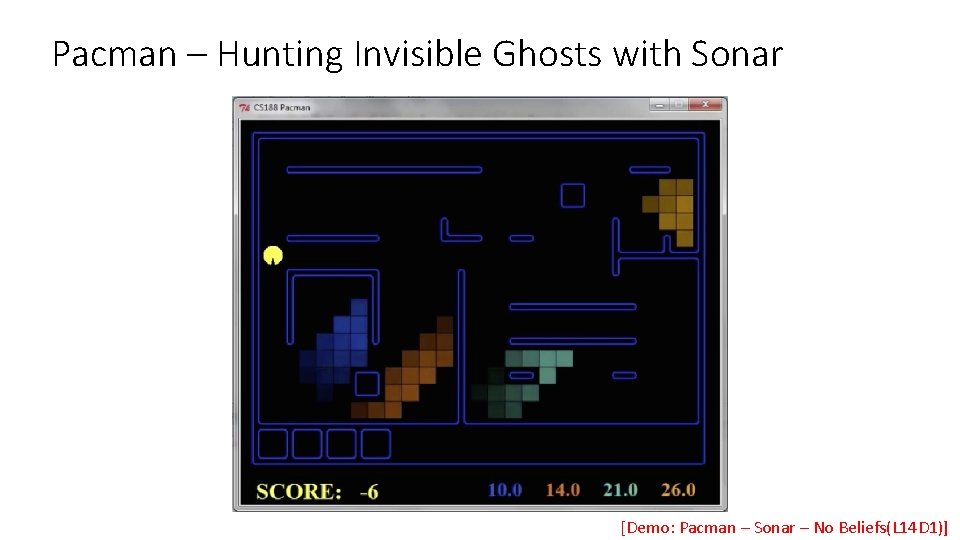
Pacman – Hunting Invisible Ghosts with Sonar [Demo: Pacman – Sonar – No Beliefs(L 14 D 1)]

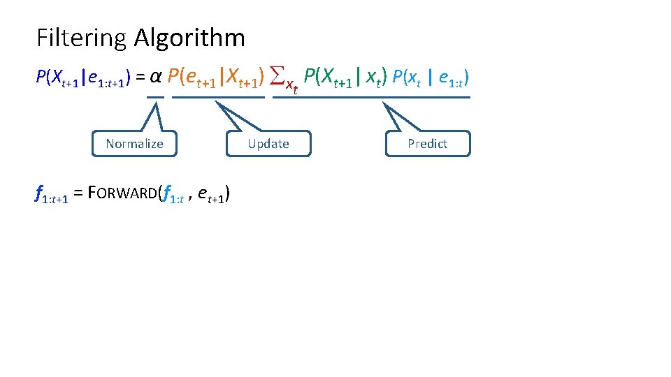
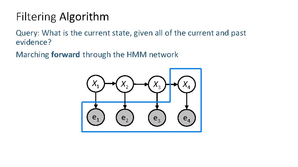
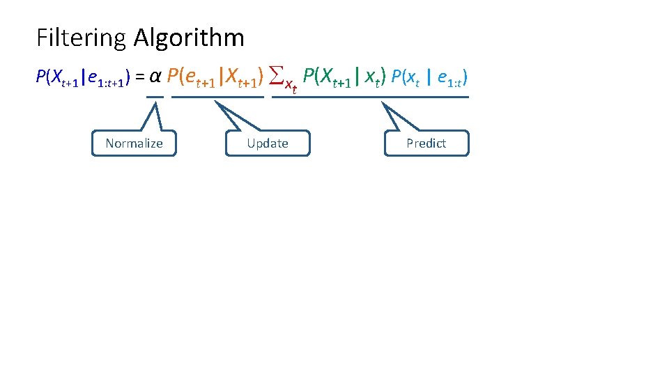
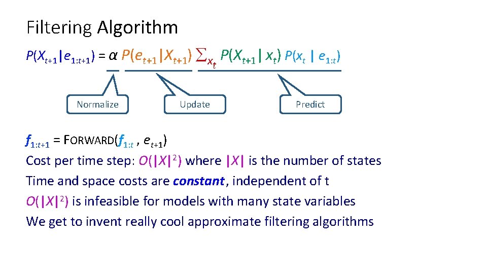
Filtering Algorithm P(Xt+1|e 1: t+1) = α P(et+1|Xt+1) x P(Xt+1| xt) P(xt | e 1: t) t Normalize f 1: t+1 = FORWARD(f 1: t , et+1) Update Predict

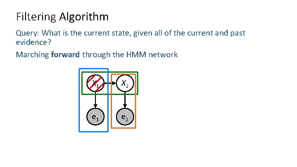
Filtering Algorithm Query: What is the current state, given all of the current and past evidence? Marching forward through the HMM network X 1 X 2 e 1 e 2

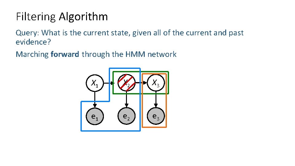
Filtering Algorithm Query: What is the current state, given all of the current and past evidence? Marching forward through the HMM network X 1 X 2 X 3 e 1 e 2 e 3

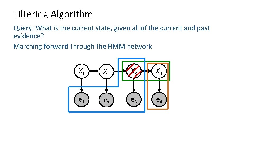
Filtering Algorithm Query: What is the current state, given all of the current and past evidence? Marching forward through the HMM network X 1 X 2 X 3 X 4 e 1 e 2 e 3 e 4

Filtering Algorithm Query: What is the current state, given all of the current and past evidence? Marching forward through the HMM network X 1 X 2 X 3 X 4 e 1 e 2 e 3 e 4

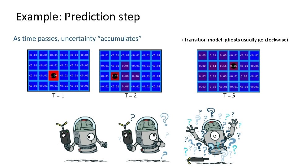
Example: Prediction step As time passes, uncertainty “accumulates” T = 1 T = 2 (Transition model: ghosts usually go clockwise) T = 5

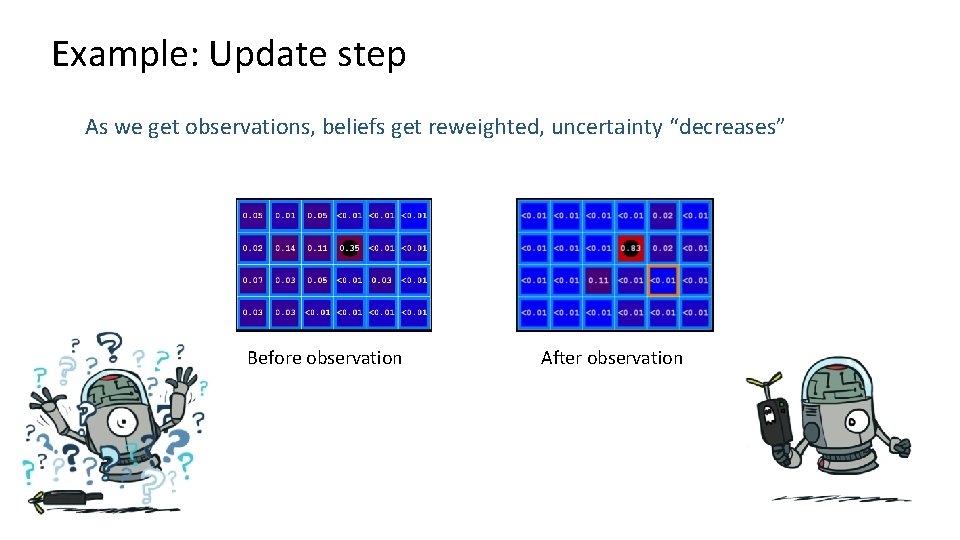
Example: Update step As we get observations, beliefs get reweighted, uncertainty “decreases” Before observation After observation

Demo Ghostbusters – Circular Dynamics -- HMM

Filtering Algorithm P(Xt+1|e 1: t+1) = α P(et+1|Xt+1) x P(Xt+1| xt) P(xt | e 1: t) t Normalize Update Predict

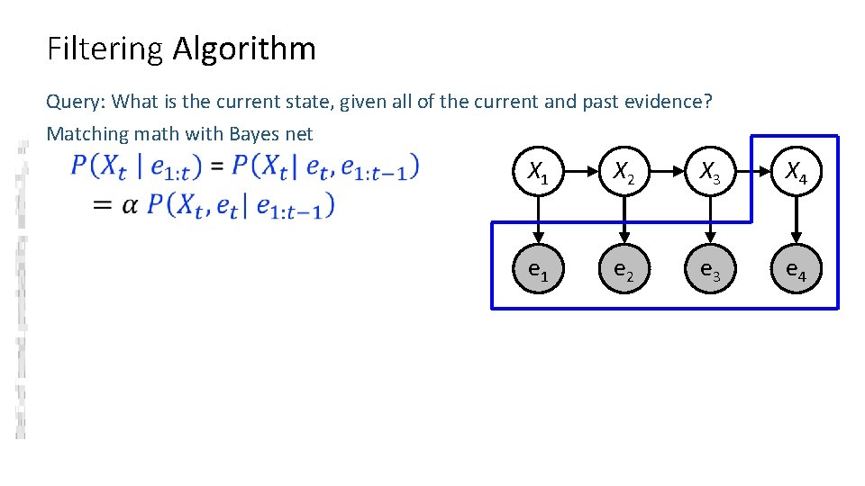
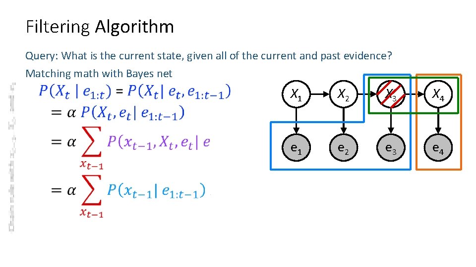
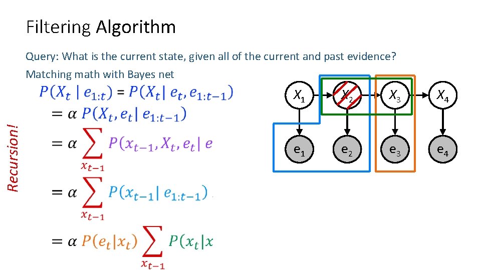
Filtering Algorithm Query: What is the current state, given all of the current and past evidence? Matching math with Bayes net X 1 X 2 X 3 X 4 e 1 e 2 e 3 e 4

Filtering Algorithm Query: What is the current state, given all of the current and past evidence? Matching math with Bayes net X 1 X 2 X 3 X 4 e 1 e 2 e 3 e 4

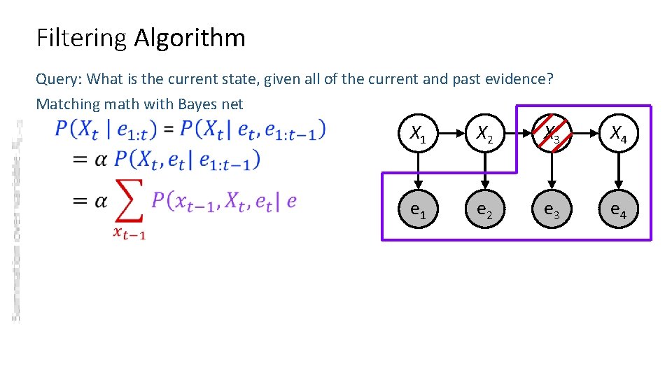
Filtering Algorithm Query: What is the current state, given all of the current and past evidence? Matching math with Bayes net X 1 X 2 X 3 X 4 e 1 e 2 e 3 e 4

Filtering Algorithm Query: What is the current state, given all of the current and past evidence? Matching math with Bayes net X 1 X 2 X 3 X 4 e 1 e 2 e 3 e 4

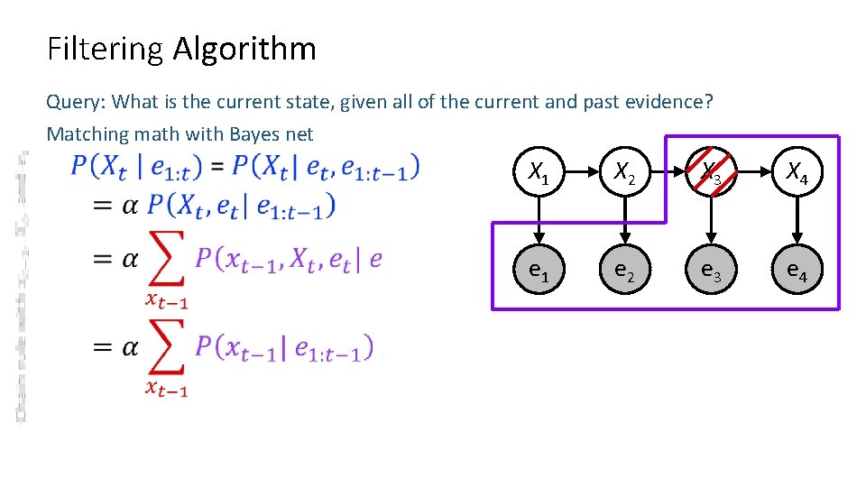
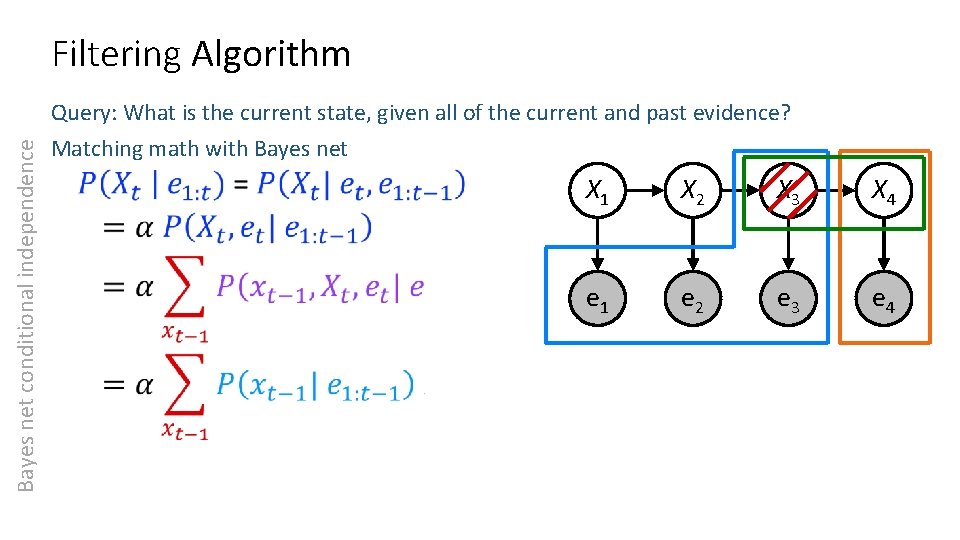
Bayes net conditional independence Filtering Algorithm Query: What is the current state, given all of the current and past evidence? Matching math with Bayes net X 1 X 2 X 3 X 4 e 1 e 2 e 3 e 4

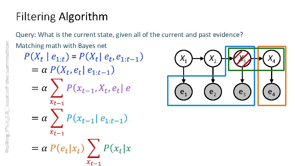
Filtering Algorithm Query: What is the current state, given all of the current and past evidence? Matching math with Bayes net X 1 X 2 X 3 X 4 e 1 e 2 e 3 e 4

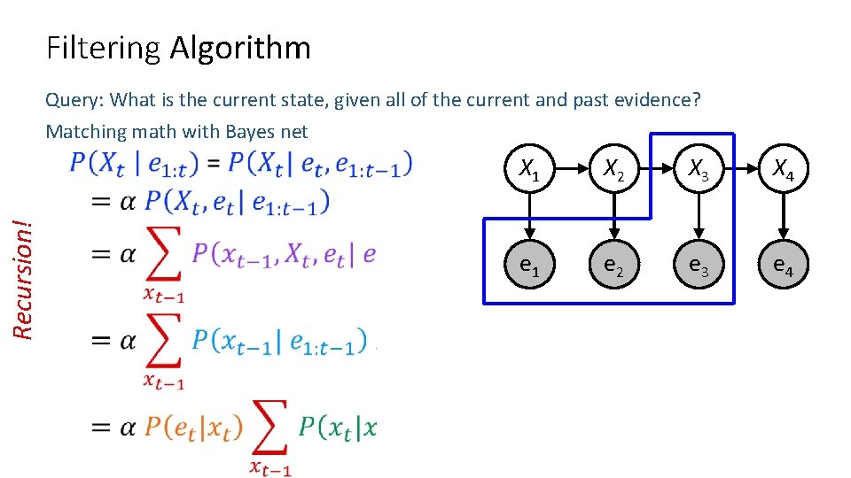
Filtering Algorithm Query: What is the current state, given all of the current and past evidence? Matching math with Bayes net Recursion! X 1 X 2 X 3 X 4 e 1 e 2 e 3 e 4

Filtering Algorithm Query: What is the current state, given all of the current and past evidence? Matching math with Bayes net Recursion! X 1 X 2 X 3 X 4 e 1 e 2 e 3 e 4

Filtering Algorithm P(Xt+1|e 1: t+1) = α P(et+1|Xt+1) x P(Xt+1| xt) P(xt | e 1: t) t Normalize Update Predict f 1: t+1 = FORWARD(f 1: t , et+1) Cost per time step: O(|X|2) where |X| is the number of states Time and space costs are constant, independent of t O(|X|2) is infeasible for models with many state variables We get to invent really cool approximate filtering algorithms

Particle Filtering

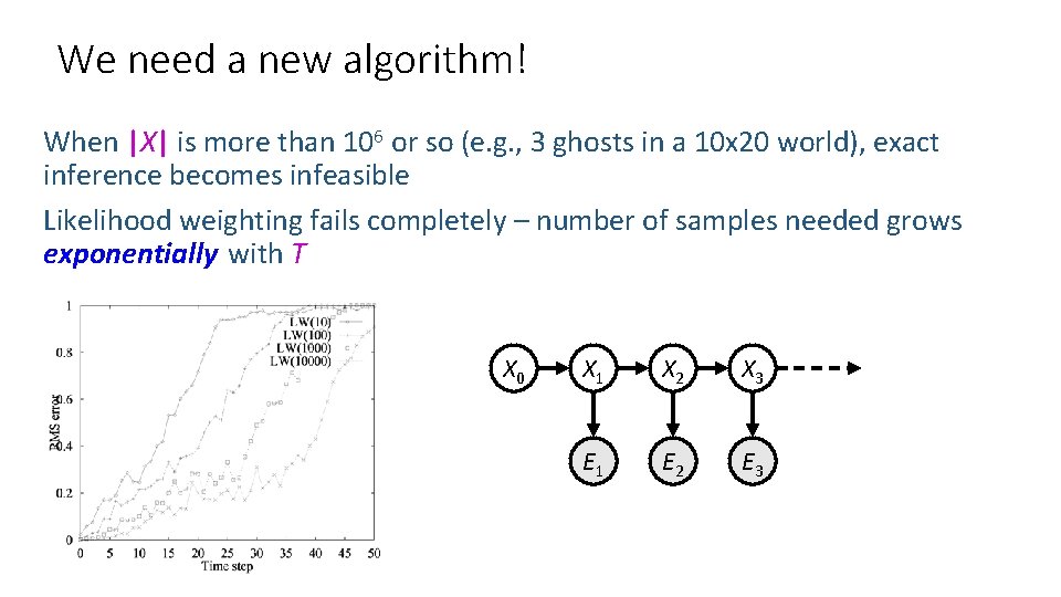
We need a new algorithm! When |X| is more than 106 or so (e. g. , 3 ghosts in a 10 x 20 world), exact inference becomes infeasible Likelihood weighting fails completely – number of samples needed grows exponentially with T X 0 X 1 X 2 X 3 E 1 E 2 E 3

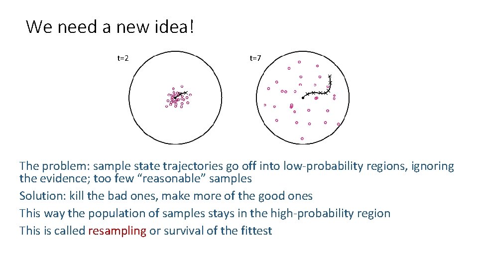
We need a new idea! t=2 t=7 The problem: sample state trajectories go off into low-probability regions, ignoring the evidence; too few “reasonable” samples Solution: kill the bad ones, make more of the good ones This way the population of samples stays in the high-probability region This is called resampling or survival of the fittest

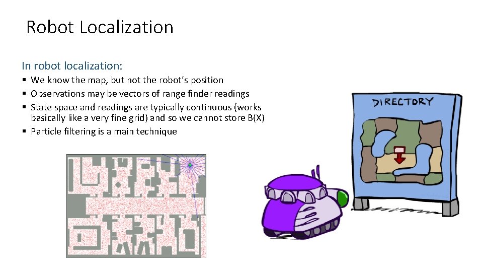
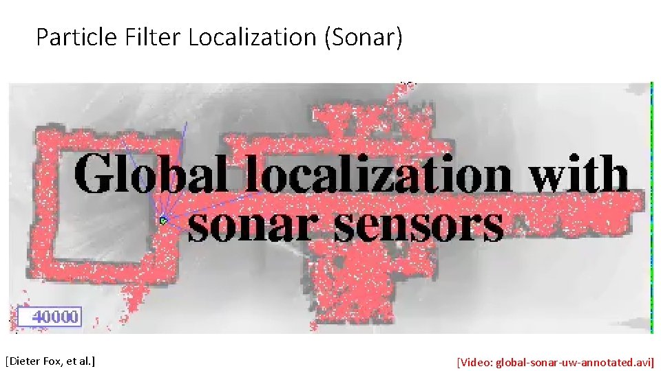
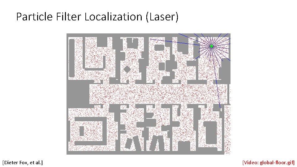
Robot Localization In robot localization: § We know the map, but not the robot’s position § Observations may be vectors of range finder readings § State space and readings are typically continuous (works basically like a very fine grid) and so we cannot store B(X) § Particle filtering is a main technique

Particle Filter Localization (Sonar) [Dieter Fox, et al. ] [Video: global-sonar-uw-annotated. avi]

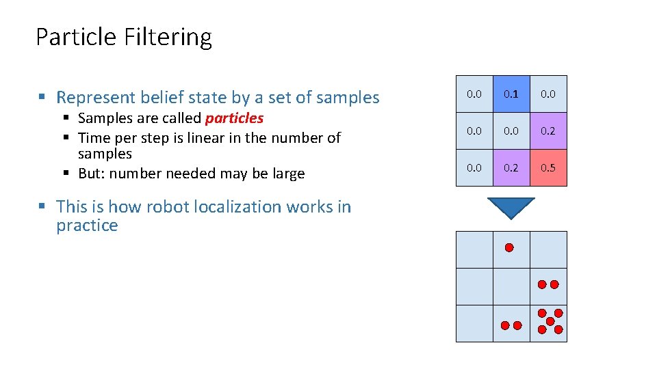
Particle Filtering § Represent belief state by a set of samples § Samples are called particles § Time per step is linear in the number of samples § But: number needed may be large § This is how robot localization works in practice 0. 0 0. 1 0. 0 0. 2 0. 5

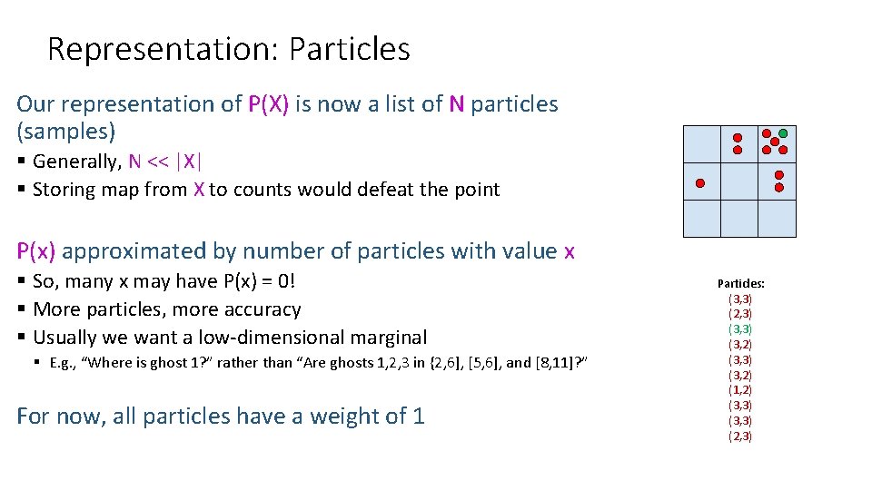
Representation: Particles Our representation of P(X) is now a list of N particles (samples) § Generally, N << |X| § Storing map from X to counts would defeat the point P(x) approximated by number of particles with value x § So, many x may have P(x) = 0! § More particles, more accuracy § Usually we want a low-dimensional marginal § E. g. , “Where is ghost 1? ” rather than “Are ghosts 1, 2, 3 in {2, 6], [5, 6], and [8, 11]? ” For now, all particles have a weight of 1 Particles: (3, 3) (2, 3) (3, 3) (3, 2) (3, 3) (3, 2) (1, 2) (3, 3) (2, 3)

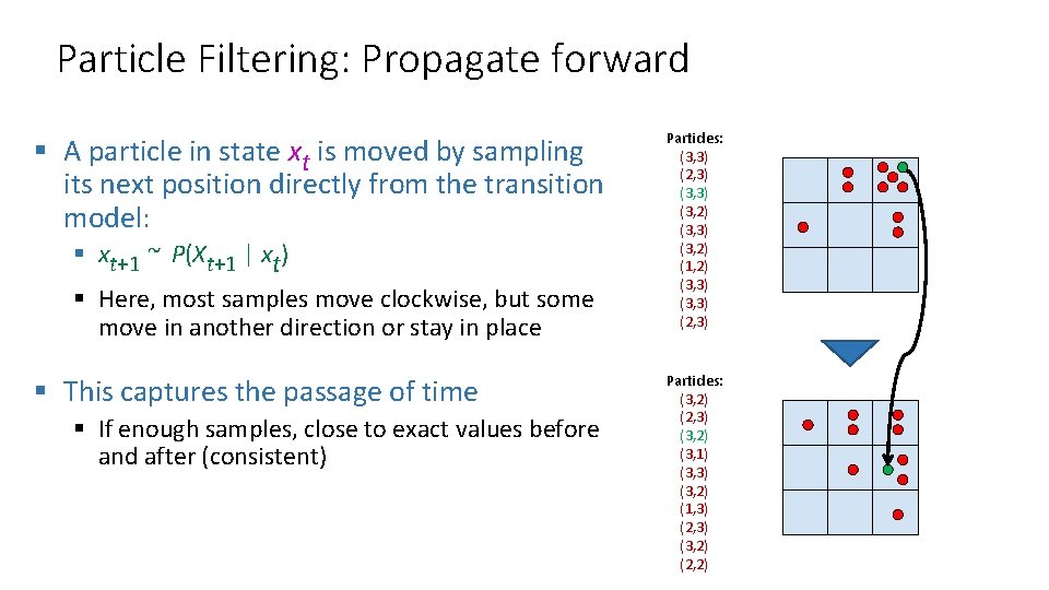
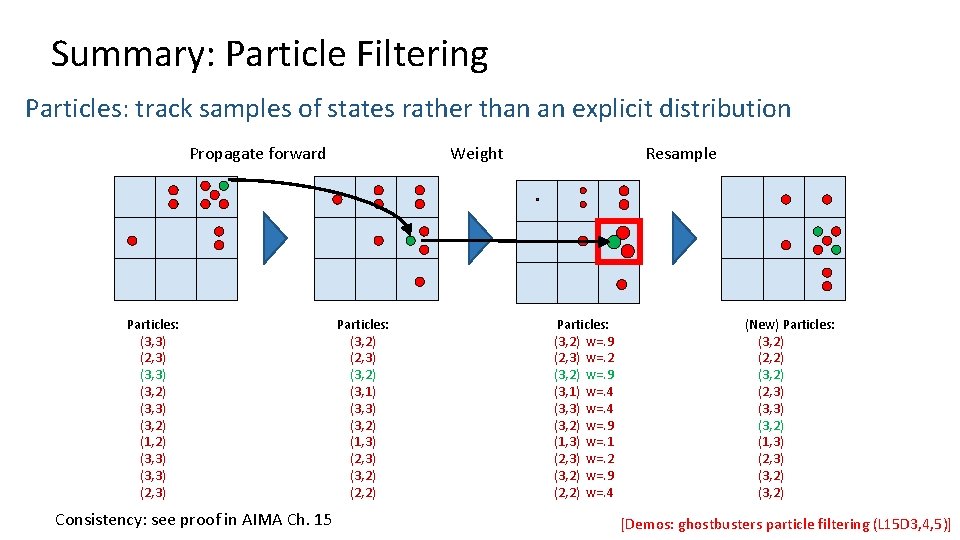
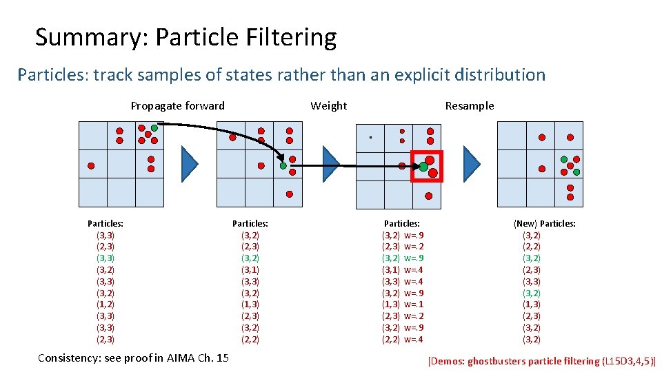
Particle Filtering: Propagate forward § A particle in state xt is moved by sampling its next position directly from the transition model: § xt+1 ~ P(Xt+1 | xt) § Here, most samples move clockwise, but some move in another direction or stay in place § This captures the passage of time § If enough samples, close to exact values before and after (consistent) Particles: (3, 3) (2, 3) (3, 3) (3, 2) (3, 3) (3, 2) (1, 2) (3, 3) (2, 3) Particles: (3, 2) (2, 3) (3, 2) (3, 1) (3, 3) (3, 2) (1, 3) (2, 3) (3, 2) (2, 2)

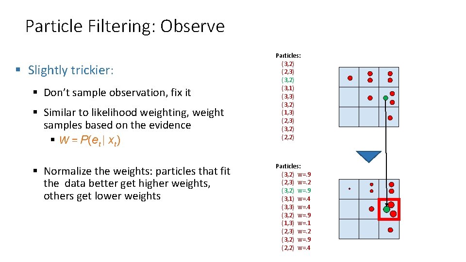
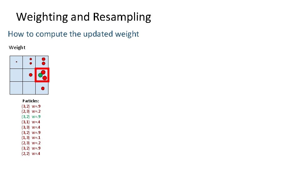
Particle Filtering: Observe § Slightly trickier: § Don’t sample observation, fix it § Similar to likelihood weighting, weight samples based on the evidence § W = P(et| xt) § Normalize the weights: particles that fit the data better get higher weights, others get lower weights Particles: (3, 2) (2, 3) (3, 2) (3, 1) (3, 3) (3, 2) (1, 3) (2, 3) (3, 2) (2, 2) Particles: (3, 2) w=. 9 (2, 3) w=. 2 (3, 2) w=. 9 (3, 1) w=. 4 (3, 3) w=. 4 (3, 2) w=. 9 (1, 3) w=. 1 (2, 3) w=. 2 (3, 2) w=. 9 (2, 2) w=. 4

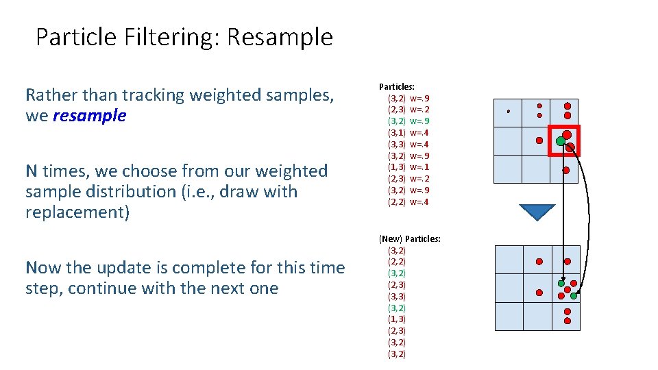
Particle Filtering: Resample Rather than tracking weighted samples, we resample N times, we choose from our weighted sample distribution (i. e. , draw with replacement) Now the update is complete for this time step, continue with the next one Particles: (3, 2) w=. 9 (2, 3) w=. 2 (3, 2) w=. 9 (3, 1) w=. 4 (3, 3) w=. 4 (3, 2) w=. 9 (1, 3) w=. 1 (2, 3) w=. 2 (3, 2) w=. 9 (2, 2) w=. 4 (New) Particles: (3, 2) (2, 2) (3, 2) (2, 3) (3, 2) (1, 3) (2, 3) (3, 2)

Summary: Particle Filtering Particles: track samples of states rather than an explicit distribution Propagate forward Particles: (3, 3) (2, 3) (3, 3) (3, 2) (3, 3) (3, 2) (1, 2) (3, 3) (2, 3) Consistency: see proof in AIMA Ch. 15 Weight Particles: (3, 2) (2, 3) (3, 2) (3, 1) (3, 3) (3, 2) (1, 3) (2, 3) (3, 2) (2, 2) Resample Particles: (3, 2) w=. 9 (2, 3) w=. 2 (3, 2) w=. 9 (3, 1) w=. 4 (3, 3) w=. 4 (3, 2) w=. 9 (1, 3) w=. 1 (2, 3) w=. 2 (3, 2) w=. 9 (2, 2) w=. 4 (New) Particles: (3, 2) (2, 2) (3, 2) (2, 3) (3, 2) (1, 3) (2, 3) (3, 2) [Demos: ghostbusters particle filtering (L 15 D 3, 4, 5)]

Summary: Particle Filtering Particles: track samples of states rather than an explicit distribution Propagate forward Particles: (3, 3) (2, 3) (3, 3) (3, 2) (3, 3) (3, 2) (1, 2) (3, 3) (2, 3) Consistency: see proof in AIMA Ch. 15 Weight Particles: (3, 2) (2, 3) (3, 2) (3, 1) (3, 3) (3, 2) (1, 3) (2, 3) (3, 2) (2, 2) Resample Particles: (3, 2) w=. 9 (2, 3) w=. 2 (3, 2) w=. 9 (3, 1) w=. 4 (3, 3) w=. 4 (3, 2) w=. 9 (1, 3) w=. 1 (2, 3) w=. 2 (3, 2) w=. 9 (2, 2) w=. 4 (New) Particles: (3, 2) (2, 2) (3, 2) (2, 3) (3, 2) (1, 3) (2, 3) (3, 2) [Demos: ghostbusters particle filtering (L 15 D 3, 4, 5)]

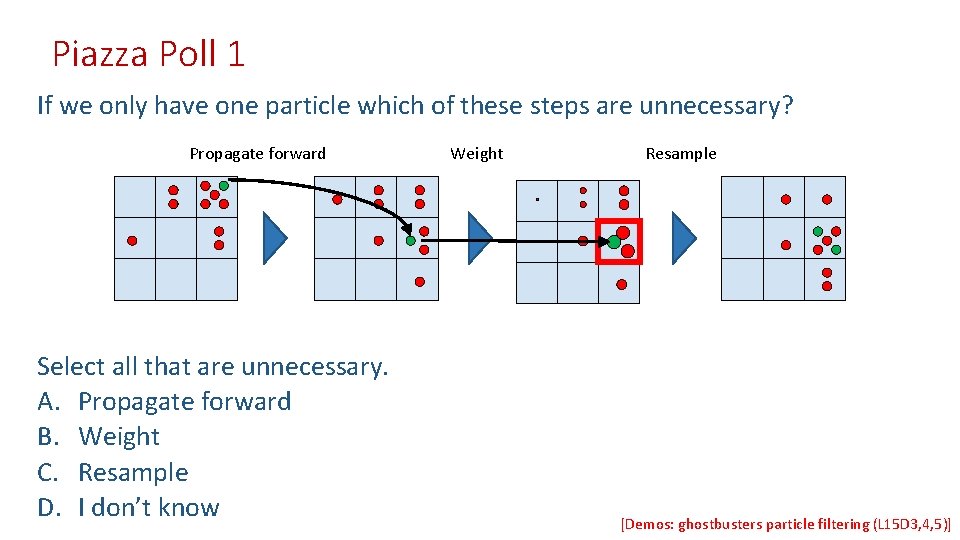
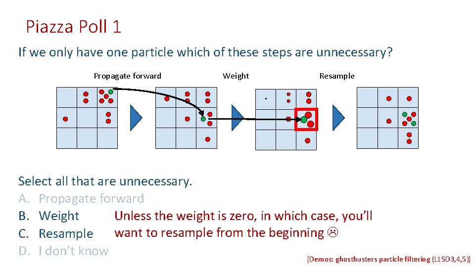
Piazza Poll 1 If we only have one particle which of these steps are unnecessary? Propagate forward Select all that are unnecessary. A. Propagate forward B. Weight C. Resample D. I don’t know Weight Resample [Demos: ghostbusters particle filtering (L 15 D 3, 4, 5)]

Piazza Poll 1 If we only have one particle which of these steps are unnecessary? Propagate forward Weight Resample Select all that are unnecessary. A. Propagate forward B. Weight Unless the weight is zero, in which case, you’ll C. Resample want to resample from the beginning D. I don’t know [Demos: ghostbusters particle filtering (L 15 D 3, 4, 5)]

Weighting and Resampling How to compute the updated weight Weight Particles: (3, 2) w=. 9 (2, 3) w=. 2 (3, 2) w=. 9 (3, 1) w=. 4 (3, 3) w=. 4 (3, 2) w=. 9 (1, 3) w=. 1 (2, 3) w=. 2 (3, 2) w=. 9 (2, 2) w=. 4

Particle Filter Localization (Laser) [Dieter Fox, et al. ] [Video: global-floor. gif]

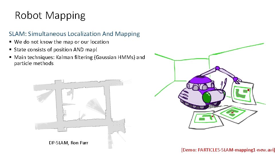
Robot Mapping SLAM: Simultaneous Localization And Mapping § We do not know the map or our location § State consists of position AND map! § Main techniques: Kalman filtering (Gaussian HMMs) and particle methods DP-SLAM, Ron Parr [Demo: PARTICLES-SLAM-mapping 1 -new. avi]

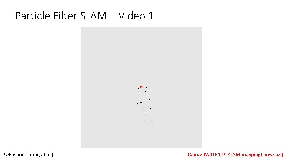
Particle Filter SLAM – Video 1 [Sebastian Thrun, et al. ] [Demo: PARTICLES-SLAM-mapping 1 -new. avi]

Particle Filter SLAM – Video 2 [Dirk Haehnel, et al. ] [Demo: PARTICLES-SLAM-fastslam. avi]